Discovering the end-to-end ML process

We have finally arrived at the main topic of this chapter. After reviewing the past and understanding the purpose of ML and how it takes its roots in mathematical data analysis, let's now get a clear picture of which steps need to be taken to create a high-quality ML model.

The following diagram shows an overview of the (sometimes recursive) steps from data to model to deployed model:

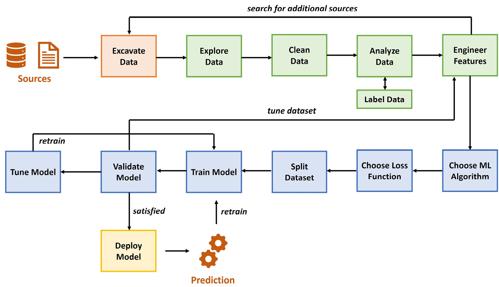
Figure 1.11 – End-to-end ML process

Looking at this flow, we can define the following distinct steps to take:

1. Excavating data and sources
2. Preparing and cleaning data
3. Defining labels and engineering features
4. Training models
5. Deploying models

These show the steps for running one single ML project. When you deal with a lot of projects and data, it becomes increasingly important to adopt some form of automation and operationalization, which is typically referred to as MLOps.

In this section, we will give an overview of each of these steps, including MLOps and its importance, and explain in which chapters we will delve deeper into the corresponding topic. Before we start going through those steps, reflect on the following question:

As a percentage, how much time would you put aside for each of those steps?

After you are done, have a look at the following screenshot, which shows you the typical time investment required for those tasks:

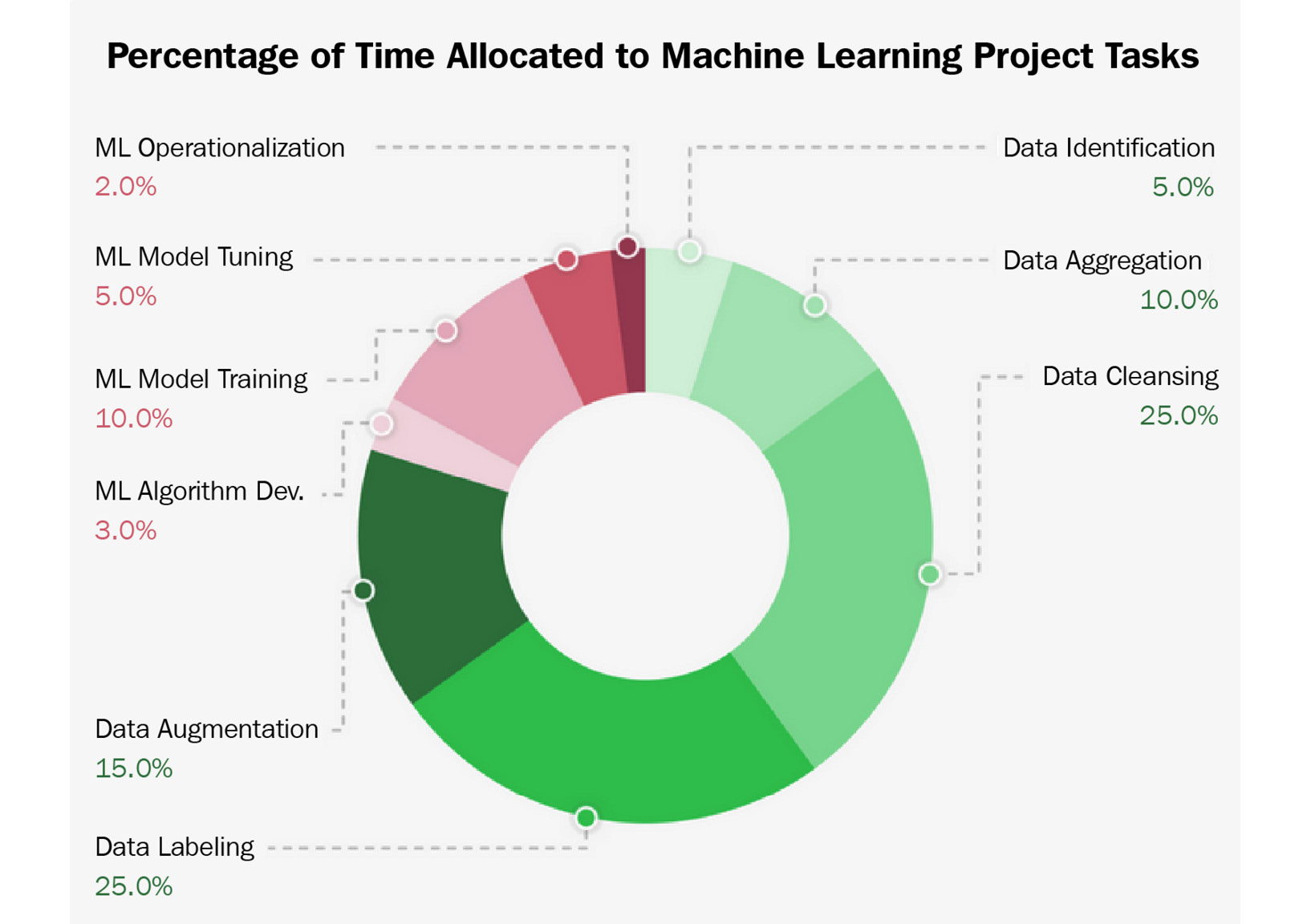
Figure 1.12 – ML time invested

Was your guess reasonably close to this? You might be surprised that only 20% of the time, you will work on something that has to do with the actual training and deployment of ML models. Therefore, you should take the next point to heart.

Important Note

In an ML project, you should spend most of your time taking apart your datasets and finding other useful data sources.

Failure to do so will have ramifications on the quality of your model and its performance. Now, having said that, let's go through the steps one by one, starting with where to source your data from.

Excavating data and sources

When you start an ML project, you probably have some outcome in mind, and often, you have some form of existing dataset you or your company wants to start with. This is where you start familiarizing yourself with the given data, understanding what you have and what is missing by doing analysis, which we will come back to in the following steps.

At some point, you might realize that you are missing additional—but crucial—data points to increase the quality of your results. This highly depends on what you are missing—whether it is something you or your company can obtain or whether you need to find it somewhere else. To give you some ideas, let's have a look at the following options to acquire additional data and what you should be aware of:

• In-house data sources: If you are running this project in or with a company, the first point to look is internally. Advantages of this are that it is free of charge, it is often standardized, and you should be able to find a person that knows this data and how it was obtained. Depending on the project, it might also be the only place you can acquire the required data. Disadvantages of this option are that you might not find what you are looking for, that the data is poorly documented, and that the quality might be in question due to bias in the data.
• Open data sources: Another option is to use freely available datasets. Advantages of those are that they are typically gigantic in size (terabytes (TB) of data), they cover different time periods, and they are typically well structured and documented. Disadvantages are that some data fields might be hard to understand (and the creator is not available), the quality might also vary due to bias in the data, and often when used, they require you to publish your results. Examples of this would be the National Oceanic and Atmospheric Administration (NOAA) (https://www.ncei.noaa.gov/weather-climate-links) and the European Union (EU) Open Data Portal (https://data.europa.eu/en), among many others.
• Data seller (data as a service, or DaaS): A final option would be to buy data from a data seller, either by purchasing an existing dataset or by requesting the creation of one. Advantages of this option are that it saves you time, it can give you access to an individualized dataset, and you might even get access to preprocessed data. Disadvantages are that this is expensive, you still need to do all the other following steps to make this data useful, and there might be questions concerning privacy and ethics.

Now that we have a good idea of where to get data initially or additionally, let's look at the next step: preparing and cleaning the data.

Preparing and cleaning data

As alluded to before, descriptive data exploration is without a doubt one of the most important steps in an ML project. If you want to clean data and build derived features or select an ML algorithm to predict a target variable in your dataset, then you need to understand your data first. Your data will define many of the necessary cleaning and preprocessing steps. It will define which algorithms you can choose, and it will ultimately define the performance of your predictive model.

The exploration should be done as a structured analytical process rather than a set of experimental tasks. Therefore, we will go through a checklist of data exploration tasks that you can perform as an initial step in every ML project, before starting any data cleaning, preprocessing, feature engineering, or model selection. By applying these steps, you will be able to understand the data and gain knowledge about the required preprocessing tasks.

Along with that, it will give you a good estimate of what kinds of difficulties you can expect in your prediction task, which is essential for judging the required algorithms and validation strategies. You will also gain an insight into which possible feature engineering methods could apply to your dataset and have a better understanding of how to select a good loss function.

Let's have a look at the required steps.

Storing and preparing data

Your data might come in a variety of different formats. You might work with tabular data stored in a comma-separated values (CSV) file; you might have images stored as Joint Photographic Experts Group (JPEG) or Portable Network Graphics (PNG) files, text stored in a JavaScript Object Notation (JSON) file, or audio files in MP3 or M4V format. CSV can be a good format as it is human-readable and can be parsed efficiently. You can open and browse it using any text editor.

If you work on your own, you might just store this raw data in a folder on your system, but when you are working with a cloud infrastructure or even just a company infrastructure in general, you might need some form of cloud storage. Certainly, you can just upload your raw data by hand to such storage, but often, the data you work with is coming from a live system and needs to be extracted from there. This means it might be worthwhile having a look at so-called extract-transform-load (ETL) tools that can automate this process and bring the required raw data into cloud storage.

After all of the preprocessing steps are done, you will have some form of layered data in your storage, from raw to cleaned to labeled to processed datasets.

We will dive deeper into this topic in Chapter 4, Ingesting Data and Managing Datasets. For now, just understand that we will automate this process of making data available for processing.

Cleaning data

In this step, we have a look at inconsistency and structural errors in the data itself. This step is often required for tabular data and sometimes text files, but not so much for image or audio files. For the latter, we might be able to crop images and change their brightness or contrast, but it might be required to go back to the source to create better-quality samples. The same goes for audio files.

For tabular datasets, we have much more options for processing. Let's go through what to look out for, as follows:

• Duplicates: Through mistakes in copying data or due to a combination of different data sources, you might find duplicate samples. Typically, copies can be deleted. Just make sure that these are not two different samples that look the same.
• Irrelevant information: In most cases, you will have datasets with a lot of different features, some of which will be completely unnecessary for your project. The obvious ones you should just remove in the beginning; others you will be able to remove later after analyzing the data further.
• Structural errors: This refers to the values you can see in the samples. You might run into different entries with the same meaning (such as US and United States) or simply typos. These should be standardized or cleaned up. A good way to do this is by visualizing all available values of a feature.
• Anomalies (outliers): This refers to very unlikely values for which you need to decide whether they are errors or actually true. This is typically done after analyzing the data when you know the distribution of a feature.
• Missing values: This refers to cells in your data that are either blank or have some generic value in them, such as NA or NaN. There are different ways to rectify this besides deleting entire samples. It is also prudent to wait until you have more insight from analyzing the data, as you might see better ways to replace them.

After this step, we can start analyzing the cleaned version of our dataset further.

Analyzing data

In this step, we apply our understanding of statistics to get some insights into our features and labels. This includes calculating statistical properties for each feature, visualizing them, finding correlated features, and measuring something that is called feature importance, which calculates the impact of a feature on the label, also referred to as the target variable.

Through these methods, we get ideas about relationships among features and between features and targets, which can help us to make a decision. In this decision-making process, we also start adding something vitally important—our domain knowledge. If you do not know what the data represents, you will have a hard time pruning it and choosing optimal features and samples for training.

There are a lot more techniques that can be applied in this step, including something called dimensional reduction. If you have thousands of features (a numerical representation of an image, for example), it gets very complicated for humans and even for ML processes to understand relationships. In such cases, it might be useful to map this high-dimensional sample to a two-dimensional or three-dimensional representation in the form of a vector. Through this, we can easily find similarities in different samples.

We will dive deeper into the topics of cleaning and analyzing data in Chapter 5, Performing Data Analysis and Visualization.

Having done all these steps, we will have a good understanding of the data we have at hand, and we might already know what we are missing. As the final step in preprocessing our data, we will have a look at creating and transforming features, typically referred to as feature engineering, and creating labels when missing.

Defining labels and engineering features

In the second part of the preprocessing of data, we will discuss the labeling of data and the actions we can perform on features. To perform these steps, we need the knowledge obtained through the exploratory steps we've discussed so far. Let's start by looking at labeling data.

Labeling

Let's start with a bummer: this process is very tedious. Labeling, also called annotation, is the least exciting part of an ML project yet one of the most important tasks in the whole process. The goal is to feed high-quality training data into the ML algorithms.

While proper labels greatly help to improve prediction performance, the labeling process will also help you to study the dataset in greater detail. Let me clarify that labeling data requires deep insight and understanding of the context of the dataset and the prediction process, which you should have acquired at this point. If we were, for example, aiming to predict breast cancer using computerized tomography (CT) scans, we would also need to understand how breast cancer can be detected in CT images to label the data.

Mislabeling the training data has a couple of consequences, such as label noise, which you want to avoid as it will affect the performance of every downstream process in the ML pipeline. In some cases, your labeling methodology is dependent on the chosen ML approach for a prediction problem. A good example is the difference between object detection and segmentation, both of which require completely differently labeled data.

There are some techniques and tooling available to speed up the labeling process that make use of the fact that we can use ML algorithms not only for the desired project but also to learn how to label our data. Such models start proposing labels during your manual annotation of the dataset.

Feature engineering

In a nutshell, in this step, we will start transforming the features or adding new features. Obviously, we are not doing such actions on a whim, but rather due to the knowledge we gathered in the previous steps. We might have understood, for example, that the full date and time are far too precise, and we need just the day of the week or the month. Whatever it might be, we will try to shape and extract what we need.

Typically, we will perform one of the following actions:

• Feature creation: Create new features from a given set of features or from additional information sources.
• Feature transformation: Transform single features to make them useful and stable for the utilized ML algorithm.
• Feature extraction: Create derived features from the original data.
• Feature selection: Choose the most prominent and predictive features.

We will dive deeper into labeling and the multitude of methods to apply to our features in Chapter 6, Feature Engineering and Labeling. In addition, we will have a detailed look at a more complex example of feature engineering when working with text data in an NLP project. You will find this in Chapter 7, Advanced Feature Extraction with NLP.

We conclude this step by reiterating how important the whole preprocessing data steps are and how much influence they have on the next step, where we will discuss model training. Further, we remember that we might need to come back to this after model training in case of lackluster performance of our model.

Training models

We finally reached the point where we can bring ML algorithms into play. As with data experimentation and preprocessing, training an ML model is an analytical, step-by-step process. Each step involves a thought process that evaluates the pros and cons of each algorithm according to the results of the experimentation phase. As in every other scientific process, it is recommended that you come up with a hypothesis first and verify whether this hypothesis is true afterward.

Let's look at the steps that define the process of training an ML model, as follows:

1. Define your ML task: First, we need to define the ML task we are facing, which most of the time is defined by the business decision behind your use case. Depending on the amount of labeled data, you can choose between unsupervised and supervised learning methods, as well as many other subcategories.
2. Pick a suitable model: Pick a suitable model for the chosen ML task. This might be a logistical regression, a gradient-boosted ensemble tree, or a DNN, just to name a few popular ML model choices. The choice is mainly dependent on the training (or production) infrastructure (such as Python, R, Julia, C, and so on) and the shape and type of the data.
3. Pick or implement a loss function and an optimizer: During the data experimentation phase, you should have already come up with a strategy on how to test your model performance. Hence, you should have picked a data split, loss function, and optimizer already. If you have not done so, you should at this point evaluate what you want to measure and optimize.
4. Pick a dataset split: Splitting your data into different sets—namely, training, validation, and test sets—gives you additional insights into the performance of your training and optimization process and helps you to avoid overfitting your model to your training data.
5. Train a simple model using cross-validation: When all the preceding choices are made, you can go ahead and train your ML model. Optimally, this is done as cross-validation on a training and validation set, without leaking training data into validation. After training a baseline model, it's time to interpret the error metric of the validation runs. Does it make sense? Is it as high or low as expected? Is it (hopefully) better than random and better than always predicting the most popular target?
6. Tune the model: Finally, you can either tune the outcome of the model by working with the so-called hyperparameters of a model, do model stacking or other advanced methods, or you might have to go back to the initial data and work on that before training the model again.

These are the base steps we perform when training our model. In the following section, we will give some more insights into the aforementioned steps, starting with how to choose a model.

Choosing a model

When it comes to choosing a good model for your data, it is recommended that you favor simple traditional models before going toward the more complex options. An example would be ensemble models, such as gradient-boosted tree ensembles, when training data is limited. These models perform well on a broad set of input values (ordinal, nominal, and numeric) as well as training efficiently, and they are understandable.

Tree-based ensemble models combine many weak learners into a single predictor based on decision trees. This greatly reduces the problem of the overfitting and instability aspects of a single decision tree. The output, after a few iterations using the default parameter, usually delivers great baseline results for many different applications.

In Chapter 9, Building ML Models Using Azure Machine Learning, we dedicate a complete section to training a gradient-boosted tree ensemble classifier using LightGBM, a popular tree ensemble library from Microsoft.

To capture the meaning of large amounts of complex training data, we need large parametric models. However, training parametric models with many hundreds of millions of parameters is no easy task, due to exploding and vanishing gradients, loss propagation through such a complex model, numerical instability, and normalization. In recent years, a branch of such high-parametric models achieved extremely good results through many complex tasks—namely, deep learning (DL).

DL basically spans up a multilayer ANN, where each layer is seen as a certain step in the data processing pipeline of the model.

In Chapter 10, Training Deep Neural Networks on Azure, and Chapter 12, Distributed Machine Learning on Azure, we will delve deeper into how to train large and complex DL models on single machines and on a distributed GPU cluster.

Finally, you might work with a completely different form of data, such as audio or text data. In such cases, there are specialized ways to preprocess and score this data. One of these fields would be recommendation engines, which we will discuss thoroughly in Chapter 13, Building a Recommendation Engine in Azure.

Choosing a loss function and an optimizer

As we discussed in the previous section, there are many metrics to choose from, depending on the type of training and model you want to use. After looking at the relationship between the feature and target dimensions, as well as the separability of the data, you should continue to evaluate which loss function and optimizer you will use to train your model.

Many ML practitioners don't value the importance of a proper error metric highly enough and just use what is easy, such as accuracy and RMSE. This choice is critical. Furthermore, it is useful to understand the baseline performance and the model's robustness to noise. The first can be achieved by computing the error metric using only the target variable with the highest occurrence as a prediction. This will be your baseline performance. The second can be done by modifying the random seed of your ML model and observing the changes to the error metric. This will show you which decimal place you can trust the error metric to.

Keep in mind that it is prudent to evaluate the chosen error metric and any additional metric you desire after training runs, and experiment whether others might be more beneficial.

As for the optimizer, it highly depends on the model you chose as to which options you have in this regard. Just remember the optimizer is how we get to the target, and the target is defined by the loss function.

Splitting the dataset

Once you have selected an ML model, a loss function, and an optimizer, you need to think about splitting your dataset for training. Optimally, the data should be split into three disjointed sets: a training, a validation, and a test dataset. We use multiple sets to ensure that the model generalizes well on unseen data and that the reported error metric can be trusted. Hence, you can see that dividing the data into representative sets is a task that should be performed as an analytical process. These sets are defined as follows:

• Training dataset: The subset of data used to fit/train the model.
• Validation dataset: The subset of data used to provide an evaluation during training to tune hyperparameters. The algorithm sees this data during training, but never learns from it. Therefore, it has an indirect influence on the model.
• Test dataset: The subset of data used to run an unbiased evaluation of the trained model after training.

If training data leaks into the validation or testing set, you risk overfitting the model and skewing the validation and testing results. Overfitting is a problem that you must handle besides underfitting the model. Both are defined as follows:

Underfitting versus Overfitting

An underfitted model performs purely on the data. The reasons for that are often that the model is too simplistic to understand the relationship between the features and the target variables, or that your initial data is lacking useful features. An overfitted model performs perfectly on the training dataset and purely on any other data. The reason for that is that it basically memorized the training data and is unable to generalize.

There are different discussions on what the size of these splits should be and many different further techniques to choose samples for each category, such as stratified splitting (sampling based on class distributions), temporal splitting, and group-based splitting. We will take a deeper look at these in Chapter 9, Building ML Models Using Azure Machine Learning.

Running the model training

In most cases, you will not build an ANN structure and an optimizer from scratch. You will use ready-made ML libraries, such as scikit-learn, TensorFlow, or PyTorch. Most of these frameworks and libraries are written in Python, which should therefore be the language of choice for your ML projects.

When writing your code for model training, it is a good idea to logically divide the required code into two files, as follows:

• Authoring script (authoring environment): The script that defines the environment (libraries, training location, and so on) in which the ML training will take place and the one triggering the execution script
• Execution script (execution environment): The script that only contains the actual ML training

By splitting your code in this way, you avoid updating the actual training script when your target environment changes. This will make code versioning and MLOps much cleaner.

To understand what types of class methods we might encounter in an ML library, let's have a look at a short code snippet from TensorFlow here:

model = tf.keras.models.Sequential([
  tf.keras.layers.Flatten(input_shape=(28, 28)),…])
model.compile(optimizer='adam',
              loss='sparse_categorical_crossentropy',
              metrics=['accuracy'])
model.fit(x_train, y_train, epochs=5)
model.evaluate(x_test, y_test)

Looking at this code, we see that we are using a model called Sequential that is a basic ANN defined by a sequential set of layers with one input and one output. We see in the model creation step that there are layers defined and some omitted other settings. In addition, in the compile() method, we define an optimizer, a loss function, and some additional metrics we are interested in. Finally, we see a method called fit() running on the training dataset and a method called evaluate() running on the test dataset. Now, what do these methods do exactly? Before we get to that, let's first define something.

Hyperparameters versus Parameters of a Model

There are two kinds of settings that are adjusted during model training. Settings such as the weights and the bias in an ANN are referred to as the parameters. They are changed during the training phase. Other settings—such as the activation functions and the number of layers in an ANN, the data split, the learning rate, or the chosen optimizer—are referred to as hyperparameters. Those are the meta settings we adjust before a training run.

Having this out of the way, let's define the typical methods you will encounter, as follows:

• Hyperparameter methods: These are methods used to define the characteristics of the model. They are often found in the constructor (as for the Sequential class), in a special function such as compile(), or they are part of the training method we discuss next.
• Training method: Often named fit() or train(), this is the main method that trains the parameter of the model based on the training dataset, the loss function, and the optimizer. These methods do not return any type of value—they just update the model object and its parameters.
• Test method: Often named evaluate(), transform(), score(), or predict(). In most cases, these return some form of result, as they are typically running the test dataset against the trained model.

This is the typical structure of methods you will encounter for a model in an ML library. Now that we have a good idea of how to set up our coding environment and use available ML libraries, let's look at how to tune the model after our initial training.

Tuning the model

After we have trained a simple ensemble model that performs reasonably better than the baseline model and achieves acceptable performance according to the expected performance estimated during data preparation, we can progress with optimization. This is a point we really want to emphasize. It's strongly discouraged to begin model optimization and stacking when a simple ensemble technique fails to deliver useful results. If this is the case, it would be much better to take a step back and dive deeper into data analysis and feature engineering.

Common ML optimization techniques—such as hyperparameter optimization, model stacking, and even automated machine learning (AutoML)—help you get the last 10% of performance boost out of your model.

Hyperparameter optimization concentrates on changing the initial settings of the model training to improve its final performance. Similarly, model stacking is a very common technique used to improve prediction performance by putting a combination of multiple different model types into a single stacked model. Hence, the output of each model is fed into a meta-model, which itself is trained through cross-validation and hyperparameter tuning. By combining significantly different models into a single stacked model, you can always outperform a single model.

If you decide to use any of those optimization techniques, it is advised to perform them in parallel and fully automated on a distributed cluster. After seeing too many ML practitioners manually parametrizing, tuning, and stacking models together, we want to raise this important message: optimizing ML models is boring.

It should rarely be done manually as it is much faster to perform it automatically as an end-to-end optimization process. Most of your time and effort should go into experimentation, data preparation, and feature engineering—that is, everything that cannot be easily automated and optimized using raw compute power. We will delve deeper into the topic of model tuning in Chapter 11, Hyperparameter Tuning and Automated Machine Learning.

This concludes all important topics to know about model training. Next, we will have a look at options for the deployment of ML models.

Deploying models

Once you have trained and optimized an ML model, it is ready for deployment. This step is typically referred to as inferencing or scoring a model. Many data science teams, in practice, stop here and move the model to production as a Docker image, often embedded in a REpresentational State Transfer (REST) API using Flask or similar frameworks. However, as you can imagine, this is not always the best solution, depending on your requirements. An ML or data engineer's responsibility doesn't stop here.

The deployment and operation of an ML pipeline can be best seen when testing the model on live data in production. A test is done to collect insights and data to continuously improve the model. Hence, collecting model performance over time is an essential step to guaranteeing and improving the performance of the model.

In general, we differentiate two main architectures for ML-scoring pipelines, as follows:

• Batch scoring using pipelines: An offline process where you evaluate an ML model against a batch of data. The result of this scoring technique is usually not time-critical, and the data to be scored is usually larger than the model.
• Real-time scoring using a container-based web service endpoint: This refers to a technique where we score single data inputs. This is very common in stream processing, where single events are scored in real time. It's obvious that this task is highly time-critical, and the execution is blocked until the resulting score is computed.

We will discuss these two architectures in more detail in Chapter 14, Model Deployments, Endpoints, and Operations. There, we will also investigate an efficient way of collecting runtimes, latency, and other operational metrics, as well as model performance.

The model files we create, and the previously mentioned options, are typically defined by a standard hardware architecture. As mentioned, we probably create a Docker image that is deployed to a virtual machine (VM) or a web service. What if we want to deploy our model to a highly specialized hardware environment, such as a GPU or a field-programmable gate array (FPGA)?

To explore this further, we will dive deeper into alternative deployment targets and methods in Chapter 15, Model Interoperability, Hardware Optimization, and Integrations. There, we will have a look at a framework called Open Neural Network eXchange (ONNX) that allows us to convert our model into a standardized model format to be deployed to virtually any environment. Additionally, we have a look at FPGAs and why they might be a good deployment target for ML, and finally, we will explore other Azure services such as Azure IoT Edge and Power BI for integration.

This step wraps up the end-to-end process for a single ML model. Next, we will see a short overview of how to make such ML projects operational in an enterprise-grade environment using MLOps.

Developing and operating enterprise-grade ML solutions

To operationalize ML projects requires the use of automated pipelines and development-operations (DevOps) methodologies such as continuous integration (CI) and continuous delivery/continuous deployment (CD). These combined are typically referred to as MLOps.

When looking at the steps we performed in an ML project, we can see that there are typically two major operations happening—the training of a model and the deployment of a model. As these can happen independently of one another, it is worthwhile defining two different automated pipelines, as follows:

• Training pipeline: This includes loading datasets (possibly even including an ETL pipeline), transformation, model training, and registering final models. This pipeline could be triggered by changes in the dataset or possible detected data drift in a deployed model.
• Deployment pipeline: This includes loading of models from the registry, creating and deploying Docker images, creating and deploying operational scripts, and the final deployment of the model to the target. This pipeline could be triggered by new versions of an ML model.

We will have a deep dive into ML pipelining with Azure Machine Learning in Chapter 8, Azure Machine Learning Pipelines.

Having these pipelines, we can then turn our eye on Azure DevOps besides other tooling. With that, we can build a life cycle for our ML projects defined by the following parts:

• Creating or retraining a model: Here, we use training pipelines to create or retrain our model while version-controlling the pipelines and the code.
• Deploying the model and creating scoring files and dependencies: Here, we use a deployment pipeline to deploy a specific model version while version-controlling the pipeline and the code.
• Creating an audit trail: Through CI/CD pipelines and version control, we create an audit trail for all assets ensuring integrity and compliance.
• Monitoring model in production: We monitor the performance and possible data drift, which might automatically trigger retraining of the model.

We will discuss these topics and others in more detail in Chapter 16, Bringing Models into Production with MLOps.

This concludes our discussion on the end-to-end ML process and this chapter. If you hadn't already, you should now have a good understanding of ML and what to expect in the rest of the book.