Getting data from Nasdaq Data Link

Alternative data can be anything that is considered non-market data, for example, weather data for agricultural commodities, satellite images that track oil shipments, or even customer feedback that reflects a company’s service performance. The idea behind using alternative data is to get an “informational edge” that can then be used for generating alpha. In short, alpha is a measure of performance describing an investment strategy’s, trader’s, or portfolio manager’s ability to beat the market.

Quandl was the leading provider of alternative data products for investment professionals (including quant funds and investment banks). Recently, it was acquired by Nasdaq and is now part of the Nasdaq Data Link service. The goal of the new platform is to provide a unified source of trusted data and analytics. It offers an easy way to download data, also via a dedicated Python library.

A good starting place for financial data would be the WIKI Prices database, which contains stock prices, dividends, and splits for 3,000 US publicly traded companies. The drawback of this database is that as of April 2018, it is no longer supported (meaning there is no recent data). However, for purposes of getting historical data or learning how to access the databases, it is more than enough.

We use the same example that we used in the previous recipe—we download Apple’s stock prices for the years 2011 to 2021.

Getting ready

Before downloading the data, we need to create an account at Nasdaq Data Link (https://data.nasdaq.com/) and then authenticate our email address (otherwise, an exception is likely to occur while downloading the data). We can find our personal API key in our profile (https://data.nasdaq.com/account/profile).

How to do it…

Execute the following steps to download data from Nasdaq Data Link:

1. Import the libraries:

   import pandas as pd
   import nasdaqdatalink
   

2. Authenticate using your personal API key:

   nasdaqdatalink.ApiConfig.api_key = "YOUR_KEY_HERE"
   

   You need to replace YOUR_KEY_HERE with your own API key.

3. Download the data:

   df = nasdaqdatalink.get(dataset="WIKI/AAPL",
                           start_date="2011-01-01", 
                           end_date="2021-12-31")
   

4. Inspect the downloaded data:

   print(f"Downloaded {len(df)} rows of data.")
   df.head()
   

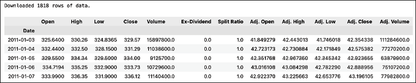
   Running the code generates the following preview of the DataFrame:

Figure 1.2: Preview of the downloaded price information

The result of the request is a DataFrame (1,818 rows) containing the daily OHLC prices, the adjusted prices, dividends, and potential stock splits. As we mentioned in the introduction, the data is limited and is only available until April 2018—the last observation actually comes from March, 27 2018.

How it works…

The first step after importing the required libraries was authentication using the API key. When providing the dataset argument, we used the following structure: DATASET/TICKER.

Some additional details on the get function are:

• We can specify multiple datasets at once using a list such as ["WIKI/AAPL", "WIKI/MSFT"].
• The collapse argument can be used to define the frequency (available options are daily, weekly, monthly, quarterly, or annually).
• The transform argument can be used to carry out some basic calculations on the data prior to downloading. For example, we could calculate row-on-row change (diff), row-on-row percentage change (rdiff), or cumulative sum (cumul) or scale the series to start at 100 (normalize). Naturally, we can easily do the very same operation using pandas.

There’s more...

Nasdaq Data Link distinguishes two types of API calls for downloading data. The get function we used before is classified as a time-series API call. We can also use the tables API call with the get_table function.

1. Download the data for multiple tickers using the get_table function:

   COLUMNS = ["ticker", "date", "adj_close"]
   df = nasdaqdatalink.get_table("WIKI/PRICES", 
                                 ticker=["AAPL", "MSFT", "INTC"], 
                                 qopts={"columns": COLUMNS}, 
                                 date={"gte": "2011-01-01", 
                                       "lte": "2021-12-31"}, 
                                 paginate=True)
   df.head()
   

2. Running the code generates the following preview of the DataFrame:

   

   Figure 1.3: Preview of the downloaded price data

   This function call is a bit more complex than the one we did with the get function. We first specified the table we want to use. Then, we provided a list of tickers. As the next step, we specified which columns of the table we were interested in. We also provided the range of dates, where gte stands for greater than or equal to, while lte is less than or equal to. Lastly, we also indicated we wanted to use pagination. The tables API is limited to 10,000 rows per call. However, by using paginate=True in the function call we extend the limit to 1,000,000 rows.

3. Pivot the data from long format to wide:

   df = df.set_index("date")
   df_wide = df.pivot(columns="ticker")
   df_wide.head()
   

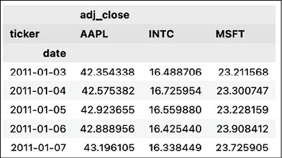
   Running the code generates the following preview of the DataFrame:

Figure 1.4: Preview of the pivoted DataFrame

The output of the get_tables function is in the long format. However, to make our analyses easier, we might be interested in the wide format. To reshape the data, we first set the date column as an index and then used the pivot method of a pd.DataFrame.

See also

• https://docs.data.nasdaq.com/docs/python—the documentation of the nasdaqdatalink library for Python.
• https://data.nasdaq.com/publishers/zacks—Zacks Investment Research is a provider of various financial data that might be relevant for your projects. Please bear in mind that the data is not free (you can always get a preview of the data before purchasing access).
• https://data.nasdaq.com/publishers—a list of all the available data providers.