We'll continue along a similar line to the previous section, in discussing classical statistical methods, but now in a new context. This section focuses on the mean of data that is quantitative, and not necessarily binary. We will demonstrate how to construct confidence intervals for the population mean, as well as several statistical tests that we can perform. Bear in mind throughout this section that we want to infer from a sample mean properties about a theoretical, unseen, yet fixed, population mean. We also want to compare the means of multiple populations, so as to determine whether they are the same or not.

When we assume that the population is a normal distribution, otherwise known as a classic bell curve, then we may use confidence intervals constructed using the t-distribution. These confidence intervals assume a normal distribution but tend to work well for large sample sizes even if the data is not normally distributed. In other words, these intervals tend to be robust. Unfortunately, statsmodels does not have a stable function with an easy user interface for competing these confidence intervals; however, there is a function, called _tconfint_generic(), that can compute them. You need to supply a lot of what this function needs to compute the confidence interval yourself. This means supplying the sample mean, the standard error of the mean, and the degrees of freedom, as shown in the following diagram:

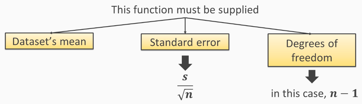
As this looks like an unstable function, this procedure could change in future versions of statsmodels.

Consider the following scenario—you are employed by a company that fabricates chips and other electronic components. The company wants you to investigate the resistors that it uses in producing its components. In particular, while the resistors used by the company are labeled with a particular resistance, the company wants to ensure that the manufacturer of the resistors produces high-quality products. In particular, when they label a resistor as having 1,000 Ω, they want to know that resistors of that type do, in fact, have 1,000 Ω, on average:

1. Let's first import NumPy, and then define our dataset in an array, as follows:

2. We read in this dataset, and the mean resistance is displayed as follows:

Now, we want to know whether it is close to 0 or not. The following is the formula for the confidence interval:

Here, x is the sample mean, s is the sample distribution, α is one minus the confidence level, and t_v,p is the p^th percentile of the t-distribution with v degrees of freedom.

3. We're going to import the _tconfint_generic() function from statsmodels. The following code block contains the statement to import the function:

4. Our next step is to define all the parameters that we will assign to the function. We are going to assign our mean, standard deviation, degrees of freedom, the confidence limit, and the alternative, which is two-sided. This results in the following output:

You will notice that 1 is not in this confidence interval. This might lead you to suspect that the resistors that the supplier produces are not being properly manufactured.

We can test the null hypothesis that the population mean (often denoted by the Greek letter μ) is equal to a hypothesized number (denoted by μ₀) against an alternative hypothesis. The alternative will state that the population mean is either less than, greater than, or not equal to the mean we hypothesized. Again, if we assume that data was drawn from a normal distribution, we can use t-procedures—namely, the t-test. This test works well for non-normal data, when the sample size is large. Unfortunately, there is not a stable function in statmodels for this test; however, we can use the _tstat_generic() function, from version 0.8.0, for this test. We may need to hack it a little bit, but it can get us the p value for this test.

So, the confidence interval that you computed earlier suggests that the resistors this manufacturer is sending your company are not being properly manufactured. In fact, you believe that their resistors have a resistance level that's less than that specified. So, you'll be testing the following hypotheses:

The first hypothesis indicates that the company is telling the truth, so you assumed that at the outset. The alternative hypothesis says that the true mean is less than 1,000 Ω. So, you are going to assume that the resistance is normally distributed, and this will be your test statistic. We will now perform the hypotheses testing using the following steps:

1. Our first step is to import the _tstat_generic() function, as follows:

2. Then, we're going to define all the parameters that will be used in the function. This includes the mean of the dataset, the mean under the null hypothesis, the standard deviation, and so on. This results in the following output:

So, we compute the p value, and this p value is minuscule. So, clearly, the resistance of the resistors the manufacturer makes is less than 1,000Ω—therefore, your company is being fleeced by this manufacturer; they're not actually producing quality parts. We can also test whether two populations have the same mean, or whether their means are different in some way.

If we assume that our data was drawn from normal distributions, the t-test can be used. For this test, we can use the statsmodels function, ttest_ind(). This is a more stable function from the package, and uses a different interface. So, here, we're going to test for a common mean.

Let's assume that your company has decided to stop outsourcing resistor production, and they're experimenting with different methods so that they can start producing resistors in-house. So, they have process A and process B, and they want you to test whether the mean resistance for these two processes is the same, or whether they're different. Therefore, you feel safe, assuming again that the resistance level of resistors is normally distributed regardless of whatever manufacturing process is employed, and you don't assume that they have the same standard deviation. Thus, the test statistic is as follows:

So, let's use this test statistic to perform your test:

Our first step is to load in the data, as follows:

Our next step is to load and define the ttest_ind function, as follows:

This will give us a p value. In this case, the p value is 0.659—this is a very large p value. It suggests that we should not reject the null hypothesis, and it appears that the two processes produce resistors with the same mean level of resistance.

One-way ANOVA tests whether all groups share a common mean with their own sample. The null hypothesis assumes that all populations share the same mean, while the alternative hypothesis simply states that the null hypothesis is false. One-way ANOVA assumes that data was drawn from normal distributions with a common standard deviation. While normality can be relaxed for larger sample sizes, the assumption of common standard deviation is, in practice, more critical.

Before performing this test, let's consider doing a visual check to see whether the data has a common spread. For example, you could create side-by-side box and whisker plots. If the data does not appear to have a common standard deviation, you should not perform this test.

The f_oneway() function from SciPy can perform this test; so, let's start performing one-way ANOVA.

Your company now has multiple processes. Therefore, before you were able to return your report for the other two, you were given data for processes C, D, and E. Your company wants to test whether all of these processes have the same mean level of resistance or whether this is not true—in other words, whether one of these processes has a different mean level of resistance. So, let's get into it:

1. We will first define the data for these other processes, as follows:

2. We're going to use the f_oneway() function from SciPy to perform this test, and we can simply pass the data from each of these samples to this function, as follows:

3. This will give us the p value, which, in this case, is 0.03:

This appears to be small, so we're going to reject the null hypothesis that all processes yield resistors with the same level of resistance. It appears at least one of them has a different mean level of resistance.

This concludes our discussion of classical statistical methods for now. We will now move on to discussing Bayesian statistics.