

ARIMA Models
Autoregressive Integrated Moving Average (ARIMA) models are a class of statistical models that try to explain the behavior of a time series using its own past values. Being a class of models, ARIMA models are defined by a set of parameters (p,d,q), each one corresponding to a different component of the ARIMA model:
- Autoregressive of order p: An autoregressive model of order p (AR(p) for short) models the current time series entry as a linear combination of its last p values. The mathematical formulation is as follows:

- Autoregressive of order p: An autoregressive model of order p (AR(p) for short) models the current time series entry as a linear combination of its last p values. The mathematical formulation is as follows:
Figure 1.40: Expression for an autoregressive model of order p
Here, α is the intercept term, Y(t-i) is the lag-I term of the series with the respective coefficient βi, while ϵt is the error term (that is, the normally distributed random variable with mean 0 and variance  ).
).
- Moving average of order q: A moving average model of order q (MA(q) for short) attempts to model the current value of the time series as a linear combination of its past error terms. Mathematically speaking, it has the following formula:

Figure 1.41: Expression for the moving average model of order q
As in the autoregressive model, α represents a bias term; ϕ1,…,ϕq are parameters to be estimated in the model; and ϵt,…,ϵ(t-q) are the error terms at times t,…,t-q, respectively.
- Integrated component of order d: The integrated component represents a transformation in the original time series, in which the transformed series is obtained by getting the difference between
Yt andY(t-d), hence the following:
Figure 1.42: Expression for an integrated component of order d
The integration term is used for detrending the original time series and making it stationary. Note that we already saw this type of transformation when we subtracted the previous entry in the number of rides, that is, when we applied an integration term of order 1.
In general, when we apply an ARIMA model of order (p,d,q) to a time series, {Yt} , we obtain the following model:
- First, integrate the original time series of order d, and then obtain the new series:

Figure 1.43: Integrating the original time series
- Then, apply a combination of the AR(p) and MA(q) models, also known as the autoregressive moving average model, or ARMA(p,q), to the transformed series,
{Zt}t:
Figure 1.44: Expression for ARMA
Here, the coefficients α,β1,…,βp,ϕ1,…,ϕq are to be estimated.
A standard method for finding the parameters (p,d,q) of an ARIMA model is to compute the autocorrelation and partial autocorrelation functions (ACF and PACF for short). The autocorrelation function measures the Pearson correlation between the lagged values in a time series as a function of the lag:

Figure 1.45: Autocorrelation function as a function of the lag
In practice, the ACF measures the complete correlation between the current entry, Yt, and its past entries, lagged by k . Note that when computing the ACF(k), the correlation between Yt with all intermediate values (Y(t-1),…,Y(t-k+1)) is not removed. In order to account only for the correlation between and Y(t-k), we often refer to the PACF, which only measures the impact of Y(t-k) on Yt.
ACF and PACF are, in general, used to determine the order of integration when modeling a time series with an ARIMA model. For each lag, the correlation coefficient and level of significance are computed. In general, we aim at an integrated series, in which only the first few lags have correlation greater than the level of significance. We will demonstrate this in the following exercise.
Exercise 1.07: ACF and PACF Plots for Registered Rides
In this exercise, we will plot the autocorrelation and partial autocorrelation functions for the registered number of rides:
- Access the necessary methods for plotting the ACF and PACF contained in the Python package,
statsmodels:from statsmodels.graphics.tsaplots import plot_acf, plot_pacf
- Define a 3 x 3 grid and plot the ACF and PACF for the original series of registered rides, as well as for its first- and second-order integrated series:
fig, axes = plt.subplots(3, 3, figsize=(25, 12))
# plot original series
original = daily_rides["registered"]
axes[0,0].plot(original)
axes[0,0].set_title("Original series")
plot_acf(original, ax=axes[0,1])
plot_pacf(original, ax=axes[0,2])
# plot first order integrated series
first_order_int = original.diff().dropna()
axes[1,0].plot(first_order_int)
axes[1,0].set_title("First order integrated")
plot_acf(first_order_int, ax=axes[1,1])
plot_pacf(first_order_int, ax=axes[1,2])
# plot first order integrated series
second_order_int = first_order_int.diff().dropna()
axes[2,0].plot(first_order_int)
axes[2,0].set_title("Second order integrated")
plot_acf(second_order_int, ax=axes[2,1])
plot_pacf(second_order_int, ax=axes[2,2])
The output should be as follows:
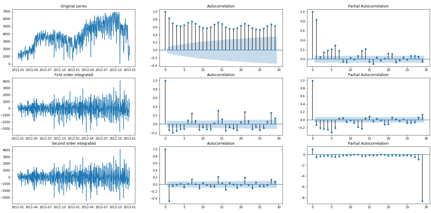
Figure 1.46: Autocorrelation and partial autocorrelation plots of registered rides
As you can see from the preceding figure, the original series exhibits several autocorrelation coefficients that are above the threshold. The first order integrated series has only a few, which makes it a good candidate for further modeling (hence, selecting an ARIMA(p,1,q) model). Finally, the second order integrated series present a large negative autocorrelation of lag 1, which, in general, is a sign of too large an order of integration.
Now focus on finding the model parameters and the coefficients for an ARIMA(p,d,q) model, based on the observed registered rides. The general approach is to try different combinations of parameters and chose the one that minimizes certain information criterion, for instance, the Akaike Information Criterion (AIC) or the Bayesian Information Criterion (BIC):
Akaike Information Criterion:

Figure 1.47: Expression for AIC
Bayesian Information Criterion:

Figure 1.48: Expression for BIC
Here,
kis the number of parameters in the selected model,nis the number of samples, and is the log likelihood. As you can see, there is no substantial difference between the two criteria and, in general, both are used. If different optimal models are selected according to the different IC, we tend to find a model in between.
 - In the following code snippet, fit an ARIMA(p,d,q) model to the registered column. Note that the
pmdarimapackage is not a standard in Anaconda; therefore, in order to install it, you need to install it via the following:conda install -c saravji pmdarima
And then perform the following:
from pmdarima import auto_arima
model = auto_arima(registered, start_p=1, start_q=1, \
                   max_p=3, max_q=3, information_criterion="aic")
print(model.summary())
Python's
pmdarimapackage has a special function that automatically finds the best parameters for an ARIMA(p,d,q) model based on the AIC. Here is the resulting model: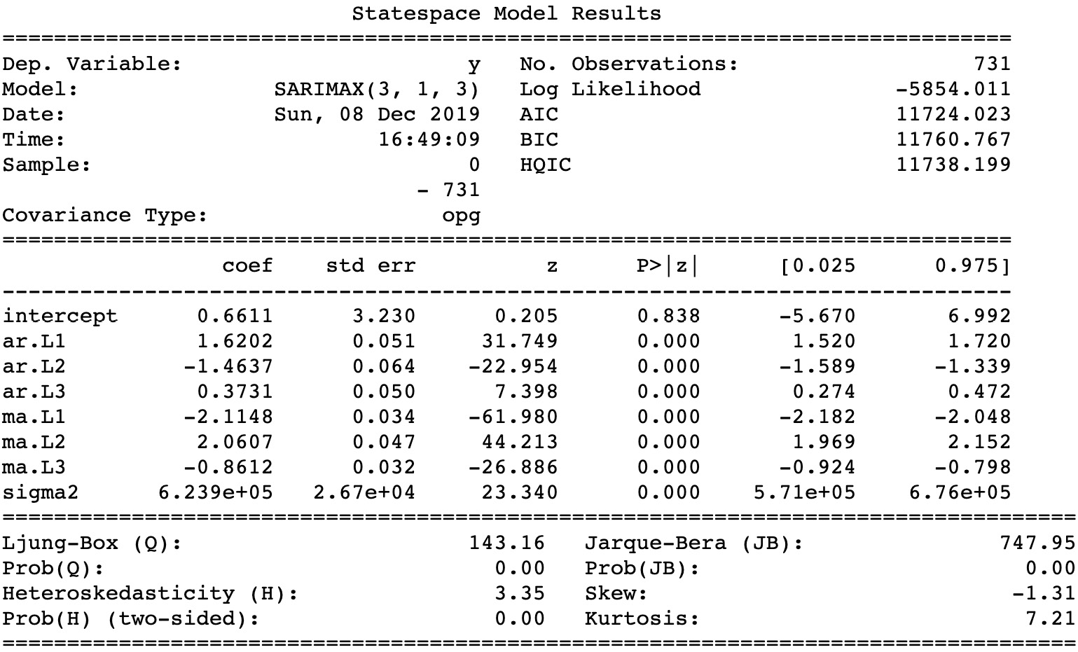
Figure 1.49: The resulting model based on AIC
As you can see, the best selected model was ARIMA(3,1,3), with the
coefcolumn containing the coefficients for the model itself. - Finally, evaluate how well the number of rides is approximated by the model by using the
model.predict_in_sample()function:# plot original and predicted values plot_data = pd.DataFrame(registered) plot_data['predicted'] = model.predict_in_sample() plot_data.plot(figsize=(12, 8)) plt.ylabel("number of registered rides") plt.title("Predicted vs actual number of rides") plt.savefig('figs/registered_arima_fit.png', format='png')The output should be as follows:
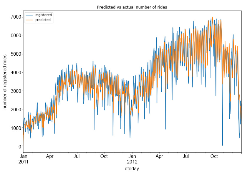
Figure 1.50: Predicted versus the actual number of registered rides
As you can see, the predicted column follows the original one quite well, although it is unable to correctly model a large number of rise and fall movements in the registered series.
Note
To access the source code for this specific section, please refer to https://packt.live/37xHHKQ.
You can also run this example online at https://packt.live/30MqcFf. You must execute the entire Notebook in order to get the desired result.
In this first chapter, we presented various techniques from data analysis and statistics, which will serve as a basis for further analysis in the next chapter, in order to improve our results and to obtain a better understanding of the problems we are about to deal with.
Activity 1.01: Investigating the Impact of Weather Conditions on Rides
In this activity, you will investigate the impact of weather conditions and their relationship with the other weather-related columns (temp, atemp, hum, and windspeed), as well as their impact on the number of registered and casual rides. The following steps will help you to perform the analysis:
- Import the initial
hourdata. - Create a new column in which
weathersitis mapped to the four categorical values specified in Exercise 1.01, Preprocessing Temporal and Weather Features. (clear,cloudy,light_rain_snow, andheavy_rain_snow). - Define a Python function that accepts as input the hour data, a column name, and a weather condition, and then returns a seaborn
regplotin which regression plots are produced between the provided column name and the registered and casual rides for the specified weather condition. - Produce a 4 x 4 plot in which each column represents a specific weather condition (
clear,cloudy,light_rain_snow, andheavy_rain_snow), and each row of the specified four columns (temp,atemp,hum, andwindspeed). A useful function for producing the plot might be thematplotlib.pyplot.subplot()function.Note
For more information on the
matplotlib.pyplot.subplot()function, refer to https://pythonspot.com/matplotlib-subplot/. - Define a second function that accepts the hour data, a column name, and a specific weather condition as an input, and then prints the Pearson's correlation and p-value between the registered and casual rides and the provided column for the specified weather condition (once when the correlation is computed between the registered rides and the specified column and once between the casual rides and the specified column).
- Iterating over the four columns (
temp,atemp,hum, andwindspeed) and four weather conditions (clear,cloudy,light_rain_snow, andheavy_rain_snow), print the correlation for each column and each weather condition by using the function defined in Step 5.The output should be as follows:
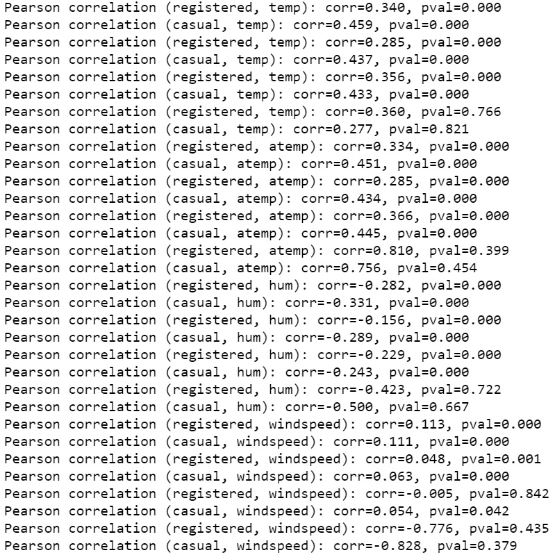
Figure 1.51: Correlation between weather and the registered/casual rides
Note
The solution for this activity can be found via this link.