-
Book Overview & Buying
-
Table Of Contents

The Data Analysis Workshop
By :
The Data Analysis Workshop
By:
Overview of this book
Businesses today operate online and generate data almost continuously. While not all data in its raw form may seem useful, if processed and analyzed correctly, it can provide you with valuable hidden insights. The Data Analysis Workshop will help you learn how to discover these hidden patterns in your data, to analyze them, and leverage the results to help transform your business.
The book begins by taking you through the use case of a bike rental shop. You'll be shown how to correlate data, plot histograms, and analyze temporal features. As you progress, you’ll learn how to plot data for a hydraulic system using the Seaborn and Matplotlib libraries, and explore a variety of use cases that show you how to join and merge databases, prepare data for analysis, and handle imbalanced data.
By the end of the book, you'll have learned different data analysis techniques, including hypothesis testing, correlation, and null-value imputation, and will have become a confident data analyst.
Table of Contents (12 chapters)
Preface

1. Bike Sharing Analysis
 Free Chapter
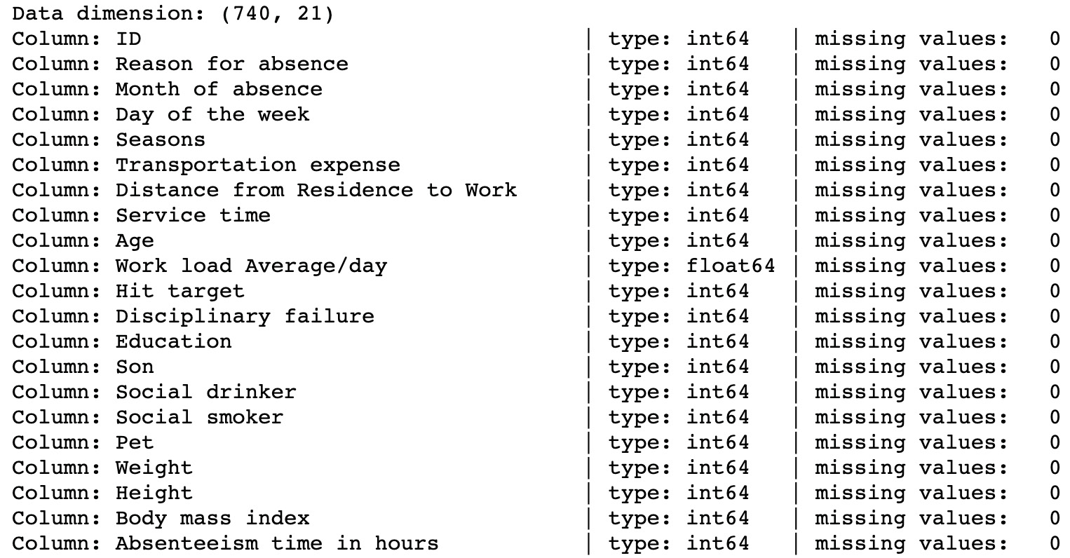
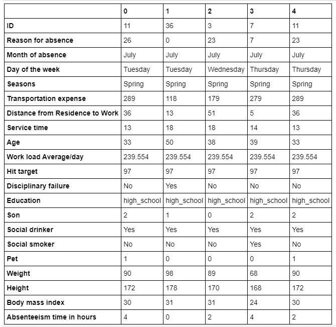
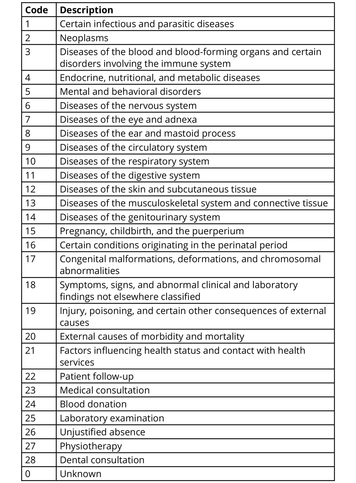
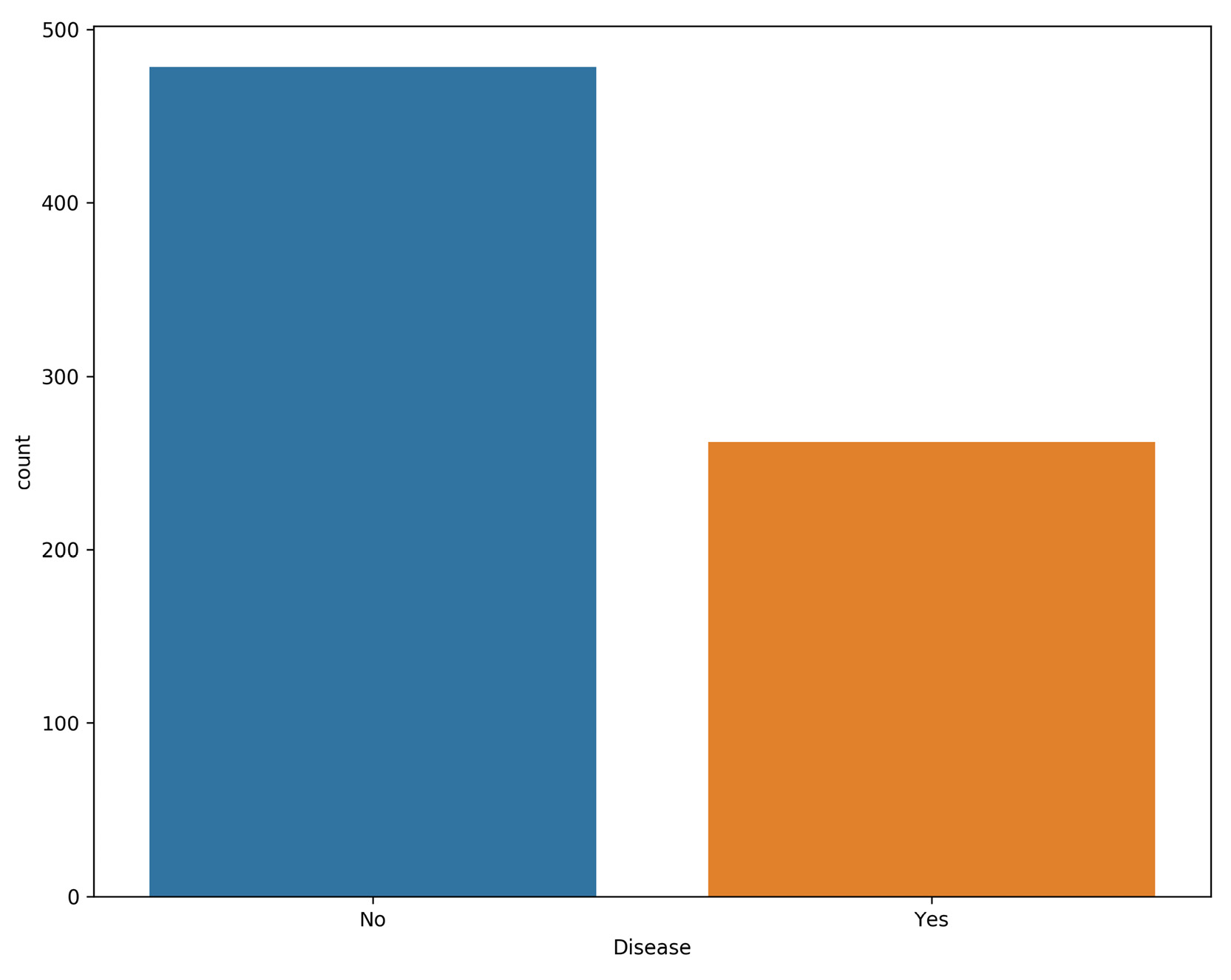
2. Absenteeism at Work
3. Analyzing Bank Marketing Campaign Data
4. Tackling Company Bankruptcy
5. Analyzing the Online Shopper's Purchasing Intention
6. Analysis of Credit Card Defaulters
7. Analyzing the Heart Disease Dataset
8. Analyzing Online Retail II Dataset
9. Analysis of the Energy Consumed by Appliances
10. Analyzing Air Quality
Appendix