

In this chapter, we will focus on:
- Implementing volume rendering using 3D texture slicing
- Implementing volume rendering using single-pass GPU ray casting
- Implementing pseudo isosurface rendering in single-pass GPU ray casting
- Implementing volume rendering using splatting
- Implementing the transfer function for volume classification
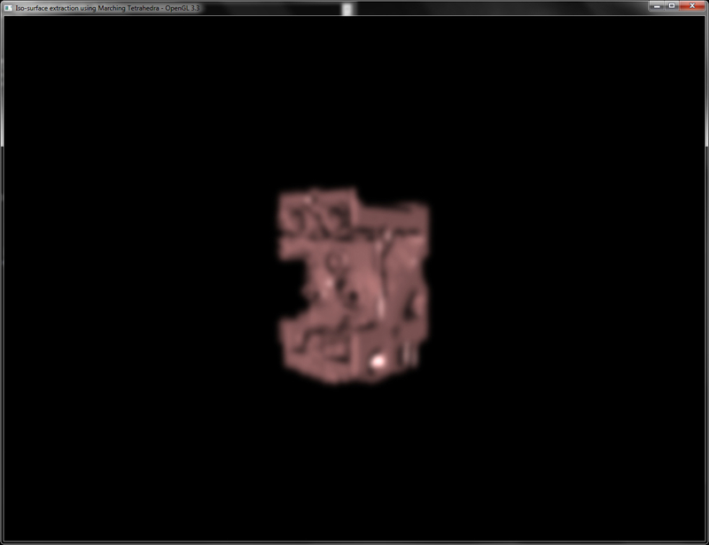
- Implementing polygonal isosurface extraction using the Marching Tetrahedra algorithm
- Implementing volumetric lighting using half-angle slicing
Volume rendering techniques are used in various domains in biomedical and engineering disciplines. They are often used in biomedical imaging to visualize the CT/MRI datasets. In mechanical engineering, they are used to visualize intermediate results from FEM simulations, flow, and structural analysis. With the advent of GPU, all of the existing models and methods of visualization were ported to GPU to harness their computational power. This chapter will detail several algorithms that are used for volume visualization on the GPU in OpenGL Version 3.3 and above. Specifically, we will look at three widely used methods including 3D texture slicing, single-pass ray casting with alpha compositing as well as isosurface rendering, and splatting.
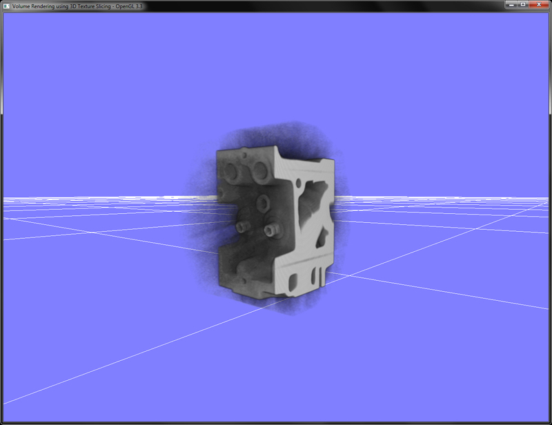
Volume rendering is a special class of rendering algorithms that allows us to portray fuzzy phenomena, such as smoke. There are numerous algorithms for volume rendering. To start our quest, we will focus on the simplest method called 3D texture slicing. This method approximates the volume-density function by slicing the dataset in front-to-back or back-to-front order and then blends the proxy slices using hardware-supported blending. Since it relies on the rasterization hardware, this method is very fast on the modern GPU.
The pseudo code for view-aligned 3D texture slicing is as follows:
- Get the current view direction vector.
- Calculate the min/max distance of unit cube vertices by doing a dot product of each unit cube vertex with the view direction vector.
- Calculate all possible intersections parameter (λ) of the plane perpendicular to the view direction with all edges of the unit cube going from the nearest to farthest vertex, using min/max distances from step 1.
- Use the intersection parameter λ (from step 3) to move in the viewing direction and find the intersection points. Three to six intersection vertices will be generated.
- Store the intersection points in the specified order to generate triangular primitives, which are the proxy geometries.
- Update the buffer object memory with the new vertices.
Let us start our recipe by following these simple steps:
- Load the volume dataset by reading the external volume datafile and passing the data into an OpenGL texture. Also enable hardware mipmap generation. Typically, the volume datafiles store densities that are obtained from using a cross-sectional imaging modality such as CT or MRI scans. Each CT/MRI scan is a 2D slice. We accumulate these slices in Z direction to obtain a 3D texture, which is simply an array of 2D textures. The densities store different material types, for example, values ranging from 0 to 20 are typically occupied by air. As we have an 8-bit unsigned dataset, we store the dataset into a local array of
GLubytetype. If we had an unsigned 16-bit dataset, we would have stored it into a local array ofGLushorttype. In case of 3D textures, in addition to theSandTparameters, we have an additional parameterRthat controls the slice we are at in the 3D texture.std::ifstream infile(volume_file.c_str(), std::ios_base::binary); if(infile.good()) { GLubyte* pData = new GLubyte[XDIM*YDIM*ZDIM]; infile.read(reinterpret_cast<char*>(pData), XDIM*YDIM*ZDIM*sizeof(GLubyte)); infile.close(); glGenTextures(1, &textureID); glBindTexture(GL_TEXTURE_3D, textureID); glTexParameteri(GL_TEXTURE_3D, GL_TEXTURE_WRAP_S, GL_CLAMP); glTexParameteri(GL_TEXTURE_3D, GL_TEXTURE_WRAP_T, GL_CLAMP); glTexParameteri(GL_TEXTURE_3D, GL_TEXTURE_WRAP_R, GL_CLAMP); glTexParameteri(GL_TEXTURE_3D, GL_TEXTURE_MAG_FILTER, GL_LINEAR); glTexParameteri(GL_TEXTURE_3D, GL_TEXTURE_MIN_FILTER, GL_LINEAR_MIPMAP_LINEAR); glTexParameteri(GL_TEXTURE_3D, GL_TEXTURE_BASE_LEVEL, 0); glTexParameteri(GL_TEXTURE_3D, GL_TEXTURE_MAX_LEVEL, 4); glTexImage3D(GL_TEXTURE_3D,0,GL_RED,XDIM,YDIM,ZDIM,0,GL_RED,GL_UNSIGNED_BYTE,pData); glGenerateMipmap(GL_TEXTURE_3D); return true; } else { return false; }The filtering parameters for 3D textures are similar to the 2D texture parameters that we have seen before. Mipmaps are collections of down-sampled versions of a texture that are used for level of detail (LOD) functionality. That is, they help to use a down-sampled version of the texture if the viewer is very far from the object on which the texture is applied. This helps improve the performance of the application. We have to specify the max number of levels (
GL_TEXTURE_MAX_LEVEL), which is the maximum number of mipmaps generated from the given texture. In addition, the base level (GL_TEXTURE_BASE_LEVEL) denotes the first level for the mipmap that is used when the object is closest. - Setup a vertex array object and a vertex buffer object to store the geometry of the proxy slices. Make sure that the buffer object usage is specified as
GL_DYNAMIC_DRAW. The initialglBufferDatacall allocates GPU memory for the maximum number of slices. ThevTextureSlicesarray is defined globally and it stores the vertices produced by texture slicing operation for triangulation. TheglBufferDatais initialized with0as the data will be filled at runtime dynamically.const int MAX_SLICES = 512; glm::vec3 vTextureSlices[MAX_SLICES*12]; glGenVertexArrays(1, &volumeVAO); glGenBuffers(1, &volumeVBO); glBindVertexArray(volumeVAO); glBindBuffer (GL_ARRAY_BUFFER, volumeVBO); glBufferData (GL_ARRAY_BUFFER, sizeof(vTextureSlices), 0, GL_DYNAMIC_DRAW); glEnableVertexAttribArray(0); glVertexAttribPointer(0, 3, GL_FLOAT, GL_FALSE,0,0); glBindVertexArray(0); - Implement slicing of volume by finding intersections of a unit cube with proxy slices perpendicular to the viewing direction. This is carried out by the
SliceVolumefunction. We use a unit cube since our data has equal size in all three axes that is, 256×256×256. If we have a non-equal sized dataset, we can scale the unit cube appropriately.//determine max and min distances glm::vec3 vecStart[12]; glm::vec3 vecDir[12]; float lambda[12]; float lambda_inc[12]; float denom = 0; float plane_dist = min_dist; float plane_dist_inc = (max_dist-min_dist)/float(num_slices); //determine vecStart and vecDir values glm::vec3 intersection[6]; float dL[12]; for(int i=num_slices-1;i>=0;i--) { for(int e = 0; e < 12; e++) { dL[e] = lambda[e] + i*lambda_inc[e]; } if ((dL[0] >= 0.0) && (dL[0] < 1.0)) { intersection[0] = vecStart[0] + dL[0]*vecDir[0]; } //like wise for all intersection points int indices[]={0,1,2, 0,2,3, 0,3,4, 0,4,5}; for(int i=0;i<12;i++) vTextureSlices[count++]=intersection[indices[i]]; } //update buffer object glBindBuffer(GL_ARRAY_BUFFER, volumeVBO); glBufferSubData(GL_ARRAY_BUFFER, 0, sizeof(vTextureSlices), &(vTextureSlices[0].x)); - In the render function, set the over blending, bind the volume vertex array object, bind the shader, and then call the
glDrawArraysfunction.glEnable(GL_BLEND); glBlendFunc(GL_SRC_ALPHA, GL_ONE_MINUS_SRC_ALPHA); glBindVertexArray(volumeVAO); shader.Use(); glUniformMatrix4fv(shader("MVP"), 1, GL_FALSE, glm::value_ptr(MVP)); glDrawArrays(GL_TRIANGLES, 0, sizeof(vTextureSlices)/sizeof(vTextureSlices[0])); shader.UnUse(); glDisable(GL_BLEND);
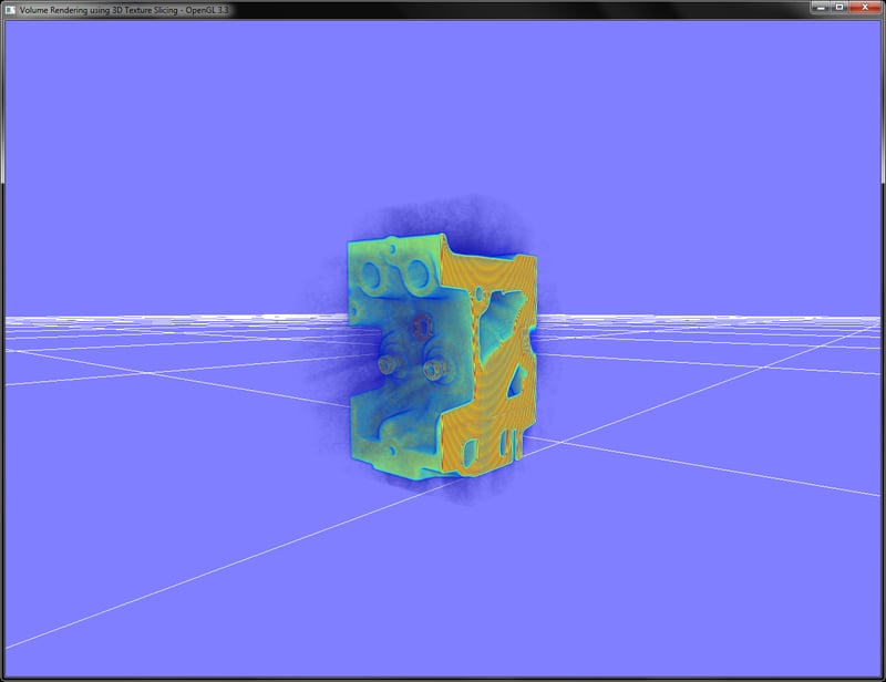
Volume rendering using 3D texture slicing approximates the volume rendering integral by alpha-blending textured slices. The first step is loading and generating a 3D texture from the volume data. After loading the volume dataset, the slicing of the volume is carried out using proxy slices. These are oriented perpendicular to the viewing direction. Moreover, we have to find the intersection of the proxy polygons with the unit cube boundaries. This is carried out by the SliceVolume function. Note that slicing is carried out only when the view is rotated.
Next, plane intersection distances are estimated for the 12 edge indices of the unit cube:
In the rendering function, the appropriate shader is bound. The vertex shader calculates the clip space position by multiplying the object space vertex position (vPosition) with the combined model view projection (MVP) matrix. It also calculates the 3D texture coordinates (vUV) for the volume data. Since we render a unit cube, the minimum vertex position will be (-0.5,-0.5,-0.5) and the maximum vertex position will be (0.5,0.5,0.5). Since our 3D texture lookup requires coordinates from (0,0,0) to (1,1,1), we add (0.5,0.5,0.5) to the object space vertex position to obtain the correct 3D texture coordinates.
The fragment shader then uses the 3D texture coordinates to sample the volume data (which is now accessed through a new sampler type sampler3D for 3D textures) to display the density. At the time of creation of the 3D texture, we specified the internal format as GL_RED (the third parameter of the glTexImage3D function). Therefore, we can now access our densities through the red channel of the texture sampler. To get a shader of grey, we set the same value for green, blue, and alpha channels as well.
In previous OpenGL versions, we would store the volume densities in a special internal format GL_INTENSITY. This is deprecated in the OpenGL3.3 core profile. So now we have to use GL_RED, GL_GREEN, GL_BLUE, or GL_ALPHA internal formats.
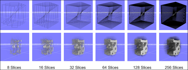
As can be seen, increasing the number of slices improves the volume rendering result. When the total number of slices goes beyond 256 slices, we do not see a significant difference in the rendering result. However, we begin to see a sharp decrease in performance as we increase the total number of slices beyond 350. This is because more geometry is transferred to the GPU and that reduces performance.
- The 3.5.2 Viewport-Aligned Slices section in Chapter 3, GPU-based Volume Rendering, Real-time Volume Graphics, AK Peters/CRC Press, page numbers 73 to 79
Chapter7/3DTextureSlicing directory.
Let us start our recipe by following these simple steps:
- Load the volume dataset by reading the external volume datafile and passing the data into an OpenGL texture. Also enable hardware mipmap generation. Typically, the volume datafiles store densities that are obtained from using a cross-sectional imaging modality such as CT or MRI scans. Each CT/MRI scan is a 2D slice. We accumulate these slices in Z direction to obtain a 3D texture, which is simply an array of 2D textures. The densities store different material types, for example, values ranging from 0 to 20 are typically occupied by air. As we have an 8-bit unsigned dataset, we store the dataset into a local array of
GLubytetype. If we had an unsigned 16-bit dataset, we would have stored it into a local array ofGLushorttype. In case of 3D textures, in addition to theSandTparameters, we have an additional parameterRthat controls the slice we are at in the 3D texture.std::ifstream infile(volume_file.c_str(), std::ios_base::binary); if(infile.good()) { GLubyte* pData = new GLubyte[XDIM*YDIM*ZDIM]; infile.read(reinterpret_cast<char*>(pData), XDIM*YDIM*ZDIM*sizeof(GLubyte)); infile.close(); glGenTextures(1, &textureID); glBindTexture(GL_TEXTURE_3D, textureID); glTexParameteri(GL_TEXTURE_3D, GL_TEXTURE_WRAP_S, GL_CLAMP); glTexParameteri(GL_TEXTURE_3D, GL_TEXTURE_WRAP_T, GL_CLAMP); glTexParameteri(GL_TEXTURE_3D, GL_TEXTURE_WRAP_R, GL_CLAMP); glTexParameteri(GL_TEXTURE_3D, GL_TEXTURE_MAG_FILTER, GL_LINEAR); glTexParameteri(GL_TEXTURE_3D, GL_TEXTURE_MIN_FILTER, GL_LINEAR_MIPMAP_LINEAR); glTexParameteri(GL_TEXTURE_3D, GL_TEXTURE_BASE_LEVEL, 0); glTexParameteri(GL_TEXTURE_3D, GL_TEXTURE_MAX_LEVEL, 4); glTexImage3D(GL_TEXTURE_3D,0,GL_RED,XDIM,YDIM,ZDIM,0,GL_RED,GL_UNSIGNED_BYTE,pData); glGenerateMipmap(GL_TEXTURE_3D); return true; } else { return false; }The filtering parameters for 3D textures are similar to the 2D texture parameters that we have seen before. Mipmaps are collections of down-sampled versions of a texture that are used for level of detail (LOD) functionality. That is, they help to use a down-sampled version of the texture if the viewer is very far from the object on which the texture is applied. This helps improve the performance of the application. We have to specify the max number of levels (
GL_TEXTURE_MAX_LEVEL), which is the maximum number of mipmaps generated from the given texture. In addition, the base level (GL_TEXTURE_BASE_LEVEL) denotes the first level for the mipmap that is used when the object is closest. - Setup a vertex array object and a vertex buffer object to store the geometry of the proxy slices. Make sure that the buffer object usage is specified as
GL_DYNAMIC_DRAW. The initialglBufferDatacall allocates GPU memory for the maximum number of slices. ThevTextureSlicesarray is defined globally and it stores the vertices produced by texture slicing operation for triangulation. TheglBufferDatais initialized with0as the data will be filled at runtime dynamically.const int MAX_SLICES = 512; glm::vec3 vTextureSlices[MAX_SLICES*12]; glGenVertexArrays(1, &volumeVAO); glGenBuffers(1, &volumeVBO); glBindVertexArray(volumeVAO); glBindBuffer (GL_ARRAY_BUFFER, volumeVBO); glBufferData (GL_ARRAY_BUFFER, sizeof(vTextureSlices), 0, GL_DYNAMIC_DRAW); glEnableVertexAttribArray(0); glVertexAttribPointer(0, 3, GL_FLOAT, GL_FALSE,0,0); glBindVertexArray(0); - Implement slicing of volume by finding intersections of a unit cube with proxy slices perpendicular to the viewing direction. This is carried out by the
SliceVolumefunction. We use a unit cube since our data has equal size in all three axes that is, 256×256×256. If we have a non-equal sized dataset, we can scale the unit cube appropriately.//determine max and min distances glm::vec3 vecStart[12]; glm::vec3 vecDir[12]; float lambda[12]; float lambda_inc[12]; float denom = 0; float plane_dist = min_dist; float plane_dist_inc = (max_dist-min_dist)/float(num_slices); //determine vecStart and vecDir values glm::vec3 intersection[6]; float dL[12]; for(int i=num_slices-1;i>=0;i--) { for(int e = 0; e < 12; e++) { dL[e] = lambda[e] + i*lambda_inc[e]; } if ((dL[0] >= 0.0) && (dL[0] < 1.0)) { intersection[0] = vecStart[0] + dL[0]*vecDir[0]; } //like wise for all intersection points int indices[]={0,1,2, 0,2,3, 0,3,4, 0,4,5}; for(int i=0;i<12;i++) vTextureSlices[count++]=intersection[indices[i]]; } //update buffer object glBindBuffer(GL_ARRAY_BUFFER, volumeVBO); glBufferSubData(GL_ARRAY_BUFFER, 0, sizeof(vTextureSlices), &(vTextureSlices[0].x)); - In the render function, set the over blending, bind the volume vertex array object, bind the shader, and then call the
glDrawArraysfunction.glEnable(GL_BLEND); glBlendFunc(GL_SRC_ALPHA, GL_ONE_MINUS_SRC_ALPHA); glBindVertexArray(volumeVAO); shader.Use(); glUniformMatrix4fv(shader("MVP"), 1, GL_FALSE, glm::value_ptr(MVP)); glDrawArrays(GL_TRIANGLES, 0, sizeof(vTextureSlices)/sizeof(vTextureSlices[0])); shader.UnUse(); glDisable(GL_BLEND);
Volume rendering using 3D texture slicing approximates the volume rendering integral by alpha-blending textured slices. The first step is loading and generating a 3D texture from the volume data. After loading the volume dataset, the slicing of the volume is carried out using proxy slices. These are oriented perpendicular to the viewing direction. Moreover, we have to find the intersection of the proxy polygons with the unit cube boundaries. This is carried out by the SliceVolume function. Note that slicing is carried out only when the view is rotated.
Next, plane intersection distances are estimated for the 12 edge indices of the unit cube:
In the rendering function, the appropriate shader is bound. The vertex shader calculates the clip space position by multiplying the object space vertex position (vPosition) with the combined model view projection (MVP) matrix. It also calculates the 3D texture coordinates (vUV) for the volume data. Since we render a unit cube, the minimum vertex position will be (-0.5,-0.5,-0.5) and the maximum vertex position will be (0.5,0.5,0.5). Since our 3D texture lookup requires coordinates from (0,0,0) to (1,1,1), we add (0.5,0.5,0.5) to the object space vertex position to obtain the correct 3D texture coordinates.
The fragment shader then uses the 3D texture coordinates to sample the volume data (which is now accessed through a new sampler type sampler3D for 3D textures) to display the density. At the time of creation of the 3D texture, we specified the internal format as GL_RED (the third parameter of the glTexImage3D function). Therefore, we can now access our densities through the red channel of the texture sampler. To get a shader of grey, we set the same value for green, blue, and alpha channels as well.
In previous OpenGL versions, we would store the volume densities in a special internal format GL_INTENSITY. This is deprecated in the OpenGL3.3 core profile. So now we have to use GL_RED, GL_GREEN, GL_BLUE, or GL_ALPHA internal formats.
As can be seen, increasing the number of slices improves the volume rendering result. When the total number of slices goes beyond 256 slices, we do not see a significant difference in the rendering result. However, we begin to see a sharp decrease in performance as we increase the total number of slices beyond 350. This is because more geometry is transferred to the GPU and that reduces performance.
- The 3.5.2 Viewport-Aligned Slices section in Chapter 3, GPU-based Volume Rendering, Real-time Volume Graphics, AK Peters/CRC Press, page numbers 73 to 79
recipe by following these simple steps:
- Load the volume dataset by reading the external volume datafile and passing the data into an OpenGL texture. Also enable hardware mipmap generation. Typically, the volume datafiles store densities that are obtained from using a cross-sectional imaging modality such as CT or MRI scans. Each CT/MRI scan is a 2D slice. We accumulate these slices in Z direction to obtain a 3D texture, which is simply an array of 2D textures. The densities store different material types, for example, values ranging from 0 to 20 are typically occupied by air. As we have an 8-bit unsigned dataset, we store the dataset into a local array of
GLubytetype. If we had an unsigned 16-bit dataset, we would have stored it into a local array ofGLushorttype. In case of 3D textures, in addition to theSandTparameters, we have an additional parameterRthat controls the slice we are at in the 3D texture.std::ifstream infile(volume_file.c_str(), std::ios_base::binary); if(infile.good()) { GLubyte* pData = new GLubyte[XDIM*YDIM*ZDIM]; infile.read(reinterpret_cast<char*>(pData), XDIM*YDIM*ZDIM*sizeof(GLubyte)); infile.close(); glGenTextures(1, &textureID); glBindTexture(GL_TEXTURE_3D, textureID); glTexParameteri(GL_TEXTURE_3D, GL_TEXTURE_WRAP_S, GL_CLAMP); glTexParameteri(GL_TEXTURE_3D, GL_TEXTURE_WRAP_T, GL_CLAMP); glTexParameteri(GL_TEXTURE_3D, GL_TEXTURE_WRAP_R, GL_CLAMP); glTexParameteri(GL_TEXTURE_3D, GL_TEXTURE_MAG_FILTER, GL_LINEAR); glTexParameteri(GL_TEXTURE_3D, GL_TEXTURE_MIN_FILTER, GL_LINEAR_MIPMAP_LINEAR); glTexParameteri(GL_TEXTURE_3D, GL_TEXTURE_BASE_LEVEL, 0); glTexParameteri(GL_TEXTURE_3D, GL_TEXTURE_MAX_LEVEL, 4); glTexImage3D(GL_TEXTURE_3D,0,GL_RED,XDIM,YDIM,ZDIM,0,GL_RED,GL_UNSIGNED_BYTE,pData); glGenerateMipmap(GL_TEXTURE_3D); return true; } else { return false; }The filtering parameters for 3D textures are similar to the 2D texture parameters that we have seen before. Mipmaps are collections of down-sampled versions of a texture that are used for level of detail (LOD) functionality. That is, they help to use a down-sampled version of the texture if the viewer is very far from the object on which the texture is applied. This helps improve the performance of the application. We have to specify the max number of levels (
GL_TEXTURE_MAX_LEVEL), which is the maximum number of mipmaps generated from the given texture. In addition, the base level (GL_TEXTURE_BASE_LEVEL) denotes the first level for the mipmap that is used when the object is closest. - Setup a vertex array object and a vertex buffer object to store the geometry of the proxy slices. Make sure that the buffer object usage is specified as
GL_DYNAMIC_DRAW. The initialglBufferDatacall allocates GPU memory for the maximum number of slices. ThevTextureSlicesarray is defined globally and it stores the vertices produced by texture slicing operation for triangulation. TheglBufferDatais initialized with0as the data will be filled at runtime dynamically.const int MAX_SLICES = 512; glm::vec3 vTextureSlices[MAX_SLICES*12]; glGenVertexArrays(1, &volumeVAO); glGenBuffers(1, &volumeVBO); glBindVertexArray(volumeVAO); glBindBuffer (GL_ARRAY_BUFFER, volumeVBO); glBufferData (GL_ARRAY_BUFFER, sizeof(vTextureSlices), 0, GL_DYNAMIC_DRAW); glEnableVertexAttribArray(0); glVertexAttribPointer(0, 3, GL_FLOAT, GL_FALSE,0,0); glBindVertexArray(0); - Implement slicing of volume by finding intersections of a unit cube with proxy slices perpendicular to the viewing direction. This is carried out by the
SliceVolumefunction. We use a unit cube since our data has equal size in all three axes that is, 256×256×256. If we have a non-equal sized dataset, we can scale the unit cube appropriately.//determine max and min distances glm::vec3 vecStart[12]; glm::vec3 vecDir[12]; float lambda[12]; float lambda_inc[12]; float denom = 0; float plane_dist = min_dist; float plane_dist_inc = (max_dist-min_dist)/float(num_slices); //determine vecStart and vecDir values glm::vec3 intersection[6]; float dL[12]; for(int i=num_slices-1;i>=0;i--) { for(int e = 0; e < 12; e++) { dL[e] = lambda[e] + i*lambda_inc[e]; } if ((dL[0] >= 0.0) && (dL[0] < 1.0)) { intersection[0] = vecStart[0] + dL[0]*vecDir[0]; } //like wise for all intersection points int indices[]={0,1,2, 0,2,3, 0,3,4, 0,4,5}; for(int i=0;i<12;i++) vTextureSlices[count++]=intersection[indices[i]]; } //update buffer object glBindBuffer(GL_ARRAY_BUFFER, volumeVBO); glBufferSubData(GL_ARRAY_BUFFER, 0, sizeof(vTextureSlices), &(vTextureSlices[0].x)); - In the render function, set the over blending, bind the volume vertex array object, bind the shader, and then call the
glDrawArraysfunction.glEnable(GL_BLEND); glBlendFunc(GL_SRC_ALPHA, GL_ONE_MINUS_SRC_ALPHA); glBindVertexArray(volumeVAO); shader.Use(); glUniformMatrix4fv(shader("MVP"), 1, GL_FALSE, glm::value_ptr(MVP)); glDrawArrays(GL_TRIANGLES, 0, sizeof(vTextureSlices)/sizeof(vTextureSlices[0])); shader.UnUse(); glDisable(GL_BLEND);
Volume rendering using 3D texture slicing approximates the volume rendering integral by alpha-blending textured slices. The first step is loading and generating a 3D texture from the volume data. After loading the volume dataset, the slicing of the volume is carried out using proxy slices. These are oriented perpendicular to the viewing direction. Moreover, we have to find the intersection of the proxy polygons with the unit cube boundaries. This is carried out by the SliceVolume function. Note that slicing is carried out only when the view is rotated.
Next, plane intersection distances are estimated for the 12 edge indices of the unit cube:
In the rendering function, the appropriate shader is bound. The vertex shader calculates the clip space position by multiplying the object space vertex position (vPosition) with the combined model view projection (MVP) matrix. It also calculates the 3D texture coordinates (vUV) for the volume data. Since we render a unit cube, the minimum vertex position will be (-0.5,-0.5,-0.5) and the maximum vertex position will be (0.5,0.5,0.5). Since our 3D texture lookup requires coordinates from (0,0,0) to (1,1,1), we add (0.5,0.5,0.5) to the object space vertex position to obtain the correct 3D texture coordinates.
The fragment shader then uses the 3D texture coordinates to sample the volume data (which is now accessed through a new sampler type sampler3D for 3D textures) to display the density. At the time of creation of the 3D texture, we specified the internal format as GL_RED (the third parameter of the glTexImage3D function). Therefore, we can now access our densities through the red channel of the texture sampler. To get a shader of grey, we set the same value for green, blue, and alpha channels as well.
In previous OpenGL versions, we would store the volume densities in a special internal format GL_INTENSITY. This is deprecated in the OpenGL3.3 core profile. So now we have to use GL_RED, GL_GREEN, GL_BLUE, or GL_ALPHA internal formats.
As can be seen, increasing the number of slices improves the volume rendering result. When the total number of slices goes beyond 256 slices, we do not see a significant difference in the rendering result. However, we begin to see a sharp decrease in performance as we increase the total number of slices beyond 350. This is because more geometry is transferred to the GPU and that reduces performance.
- The 3.5.2 Viewport-Aligned Slices section in Chapter 3, GPU-based Volume Rendering, Real-time Volume Graphics, AK Peters/CRC Press, page numbers 73 to 79
using 3D texture slicing approximates the volume rendering integral by alpha-blending textured slices. The first step is loading and generating a 3D texture from the volume data. After loading the volume dataset, the slicing of the volume is carried out using proxy slices. These are oriented perpendicular to the viewing direction. Moreover, we have to find the intersection of the proxy polygons with the unit cube boundaries. This is carried out by the SliceVolume function. Note that slicing is carried out only when the view is rotated.
Next, plane intersection distances are estimated for the 12 edge indices of the unit cube:
In the rendering function, the appropriate shader is bound. The vertex shader calculates the clip space position by multiplying the object space vertex position (vPosition) with the combined model view projection (MVP) matrix. It also calculates the 3D texture coordinates (vUV) for the volume data. Since we render a unit cube, the minimum vertex position will be (-0.5,-0.5,-0.5) and the maximum vertex position will be (0.5,0.5,0.5). Since our 3D texture lookup requires coordinates from (0,0,0) to (1,1,1), we add (0.5,0.5,0.5) to the object space vertex position to obtain the correct 3D texture coordinates.
The fragment shader then uses the 3D texture coordinates to sample the volume data (which is now accessed through a new sampler type sampler3D for 3D textures) to display the density. At the time of creation of the 3D texture, we specified the internal format as GL_RED (the third parameter of the glTexImage3D function). Therefore, we can now access our densities through the red channel of the texture sampler. To get a shader of grey, we set the same value for green, blue, and alpha channels as well.
In previous OpenGL versions, we would store the volume densities in a special internal format GL_INTENSITY. This is deprecated in the OpenGL3.3 core profile. So now we have to use GL_RED, GL_GREEN, GL_BLUE, or GL_ALPHA internal formats.
As can be seen, increasing the number of slices improves the volume rendering result. When the total number of slices goes beyond 256 slices, we do not see a significant difference in the rendering result. However, we begin to see a sharp decrease in performance as we increase the total number of slices beyond 350. This is because more geometry is transferred to the GPU and that reduces performance.
- The 3.5.2 Viewport-Aligned Slices section in Chapter 3, GPU-based Volume Rendering, Real-time Volume Graphics, AK Peters/CRC Press, page numbers 73 to 79
increasing the number of slices improves the volume rendering result. When the total number of slices goes beyond 256 slices, we do not see a significant difference in the rendering result. However, we begin to see a sharp decrease in performance as we increase the total number of slices beyond 350. This is because more geometry is transferred to the GPU and that reduces performance.
- The 3.5.2 Viewport-Aligned Slices section in Chapter 3, GPU-based Volume Rendering, Real-time Volume Graphics, AK Peters/CRC Press, page numbers 73 to 79
- Chapter 3, GPU-based Volume Rendering, Real-time Volume Graphics, AK Peters/CRC Press, page numbers 73 to 79
In this recipe, we will implement volume rendering using single-pass GPU ray casting. There are two basic approaches for doing GPU ray casting: the multi-pass approach and the single-pass approach. Both of these approaches differ in how they estimate the ray marching direction vectors. The single-pass approach uses a single fragment shader. The steps described here can be understood easily from the following diagram:

The steps required to implement single-pass GPU ray casting are as follows:
- Load the volume data from the file into a 3D OpenGL texture as in the previous recipe. Refer to the
LoadVolumefunction inChapter7/GPURaycasting/main.cppfor details. - Set up a vertex array object and a vertex buffer object to render a unit cube as follows:
glGenVertexArrays(1, &cubeVAOID); glGenBuffers(1, &cubeVBOID); glGenBuffers(1, &cubeIndicesID); glm::vec3 vertices[8]={ glm::vec3(-0.5f,-0.5f,-0.5f), glm::vec3( 0.5f,-0.5f,-0.5f),glm::vec3( 0.5f, 0.5f,-0.5f), glm::vec3(-0.5f, 0.5f,-0.5f),glm::vec3(-0.5f,-0.5f, 0.5f), glm::vec3( 0.5f,-0.5f, 0.5f),glm::vec3( 0.5f, 0.5f, 0.5f), glm::vec3(-0.5f, 0.5f, 0.5f)}; GLushort cubeIndices[36]={0,5,4,5,0,1,3,7,6,3,6,2,7,4,6,6,4,5,2,1, 3,3,1,0,3,0,7,7,0,4,6,5,2,2,5,1}; glBindVertexArray(cubeVAOID); glBindBuffer (GL_ARRAY_BUFFER, cubeVBOID); glBufferData (GL_ARRAY_BUFFER, sizeof(vertices), &(vertices[0].x), GL_STATIC_DRAW); glEnableVertexAttribArray(0); glVertexAttribPointer(0, 3, GL_FLOAT, GL_FALSE,0,0); glBindBuffer (GL_ELEMENT_ARRAY_BUFFER, cubeIndicesID); glBufferData (GL_ELEMENT_ARRAY_BUFFER, sizeof(cubeIndices), &cubeIndices[0], GL_STATIC_DRAW); glBindVertexArray(0); - In the render function, set the ray casting vertex and fragment shaders (
Chapter7/GPURaycasting/shaders/raycaster.(vert,frag)) and then render the unit cube.glEnable(GL_BLEND); glBindVertexArray(cubeVAOID); shader.Use(); glUniformMatrix4fv(shader("MVP"), 1, GL_FALSE, glm::value_ptr(MVP)); glUniform3fv(shader("camPos"), 1, &(camPos.x)); glDrawElements(GL_TRIANGLES, 36, GL_UNSIGNED_SHORT, 0); shader.UnUse(); glDisable(GL_BLEND); - From the vertex shader, in addition to the clip space position, output the 3D texture coordinates for lookup in the fragment shader. We simply offset the object space vertex positions.
smooth out vec3 vUV; void main() { gl_Position = MVP*vec4(vVertex.xyz,1); vUV = vVertex + vec3(0.5); } - In the fragment shader, use the camera position and the 3D texture coordinates to run a loop in the current viewing direction. Terminate the loop if the current sample position is outside the volume or the alpha value of the accumulated color is saturated.
vec3 dataPos = vUV; vec3 geomDir = normalize((vUV-vec3(0.5)) - camPos); vec3 dirStep = geomDir * step_size; bool stop = false; for (int i = 0; i < MAX_SAMPLES; i++) { // advance ray by step dataPos = dataPos + dirStep; // stop condition stop=dot(sign(dataPos-texMin),sign(texMax-dataPos)) < 3.0; if (stop) break; - Composite the current sample value obtained from the volume using an appropriate operator and finally return the composited color.
float sample = texture(volume, dataPos).r; float prev_alpha = sample - (sample * vFragColor.a); vFragColor.rgb = prev_alpha * vec3(sample) + vFragColor.rgb; vFragColor.a += prev_alpha; //early ray termination if( vFragColor.a>0.99) break; }
In the vertex shader (Chapter7/GPURaycasting/shaders/raycast.vert), the 3D texture coordinates are estimated using the per-vertex position of the unit cube. Since the unit cube is at origin, we add vec(0.5) to the position to bring the 3D texture coordinates to the 0 to 1 range.
The demo application for this demo shows the engine dataset rendered using single-pass GPU ray casting. The camera position can be changed using the left-mouse button and the view can be zoomed in/out by using the middle-mouse button.

- Chapter 7, GPU-based Ray Casting, Real-time Volume Graphics, AK Peters/CRC Press, page numbers 163 to 184
- Single pass Raycasting at The Little Grasshopper, http://prideout.net/blog/?p=64
Chapter7/GPURaycasting folder.
The steps required to implement single-pass GPU ray casting are as follows:
- Load the volume data from the file into a 3D OpenGL texture as in the previous recipe. Refer to the
LoadVolumefunction inChapter7/GPURaycasting/main.cppfor details. - Set up a vertex array object and a vertex buffer object to render a unit cube as follows:
glGenVertexArrays(1, &cubeVAOID); glGenBuffers(1, &cubeVBOID); glGenBuffers(1, &cubeIndicesID); glm::vec3 vertices[8]={ glm::vec3(-0.5f,-0.5f,-0.5f), glm::vec3( 0.5f,-0.5f,-0.5f),glm::vec3( 0.5f, 0.5f,-0.5f), glm::vec3(-0.5f, 0.5f,-0.5f),glm::vec3(-0.5f,-0.5f, 0.5f), glm::vec3( 0.5f,-0.5f, 0.5f),glm::vec3( 0.5f, 0.5f, 0.5f), glm::vec3(-0.5f, 0.5f, 0.5f)}; GLushort cubeIndices[36]={0,5,4,5,0,1,3,7,6,3,6,2,7,4,6,6,4,5,2,1, 3,3,1,0,3,0,7,7,0,4,6,5,2,2,5,1}; glBindVertexArray(cubeVAOID); glBindBuffer (GL_ARRAY_BUFFER, cubeVBOID); glBufferData (GL_ARRAY_BUFFER, sizeof(vertices), &(vertices[0].x), GL_STATIC_DRAW); glEnableVertexAttribArray(0); glVertexAttribPointer(0, 3, GL_FLOAT, GL_FALSE,0,0); glBindBuffer (GL_ELEMENT_ARRAY_BUFFER, cubeIndicesID); glBufferData (GL_ELEMENT_ARRAY_BUFFER, sizeof(cubeIndices), &cubeIndices[0], GL_STATIC_DRAW); glBindVertexArray(0); - In the render function, set the ray casting vertex and fragment shaders (
Chapter7/GPURaycasting/shaders/raycaster.(vert,frag)) and then render the unit cube.glEnable(GL_BLEND); glBindVertexArray(cubeVAOID); shader.Use(); glUniformMatrix4fv(shader("MVP"), 1, GL_FALSE, glm::value_ptr(MVP)); glUniform3fv(shader("camPos"), 1, &(camPos.x)); glDrawElements(GL_TRIANGLES, 36, GL_UNSIGNED_SHORT, 0); shader.UnUse(); glDisable(GL_BLEND); - From the vertex shader, in addition to the clip space position, output the 3D texture coordinates for lookup in the fragment shader. We simply offset the object space vertex positions.
smooth out vec3 vUV; void main() { gl_Position = MVP*vec4(vVertex.xyz,1); vUV = vVertex + vec3(0.5); } - In the fragment shader, use the camera position and the 3D texture coordinates to run a loop in the current viewing direction. Terminate the loop if the current sample position is outside the volume or the alpha value of the accumulated color is saturated.
vec3 dataPos = vUV; vec3 geomDir = normalize((vUV-vec3(0.5)) - camPos); vec3 dirStep = geomDir * step_size; bool stop = false; for (int i = 0; i < MAX_SAMPLES; i++) { // advance ray by step dataPos = dataPos + dirStep; // stop condition stop=dot(sign(dataPos-texMin),sign(texMax-dataPos)) < 3.0; if (stop) break; - Composite the current sample value obtained from the volume using an appropriate operator and finally return the composited color.
float sample = texture(volume, dataPos).r; float prev_alpha = sample - (sample * vFragColor.a); vFragColor.rgb = prev_alpha * vec3(sample) + vFragColor.rgb; vFragColor.a += prev_alpha; //early ray termination if( vFragColor.a>0.99) break; }
In the vertex shader (Chapter7/GPURaycasting/shaders/raycast.vert), the 3D texture coordinates are estimated using the per-vertex position of the unit cube. Since the unit cube is at origin, we add vec(0.5) to the position to bring the 3D texture coordinates to the 0 to 1 range.
The demo application for this demo shows the engine dataset rendered using single-pass GPU ray casting. The camera position can be changed using the left-mouse button and the view can be zoomed in/out by using the middle-mouse button.
- Chapter 7, GPU-based Ray Casting, Real-time Volume Graphics, AK Peters/CRC Press, page numbers 163 to 184
- Single pass Raycasting at The Little Grasshopper, http://prideout.net/blog/?p=64
implement single-pass GPU ray casting are as follows:
- Load the volume data from the file into a 3D OpenGL texture as in the previous recipe. Refer to the
LoadVolumefunction inChapter7/GPURaycasting/main.cppfor details. - Set up a vertex array object and a vertex buffer object to render a unit cube as follows:
glGenVertexArrays(1, &cubeVAOID); glGenBuffers(1, &cubeVBOID); glGenBuffers(1, &cubeIndicesID); glm::vec3 vertices[8]={ glm::vec3(-0.5f,-0.5f,-0.5f), glm::vec3( 0.5f,-0.5f,-0.5f),glm::vec3( 0.5f, 0.5f,-0.5f), glm::vec3(-0.5f, 0.5f,-0.5f),glm::vec3(-0.5f,-0.5f, 0.5f), glm::vec3( 0.5f,-0.5f, 0.5f),glm::vec3( 0.5f, 0.5f, 0.5f), glm::vec3(-0.5f, 0.5f, 0.5f)}; GLushort cubeIndices[36]={0,5,4,5,0,1,3,7,6,3,6,2,7,4,6,6,4,5,2,1, 3,3,1,0,3,0,7,7,0,4,6,5,2,2,5,1}; glBindVertexArray(cubeVAOID); glBindBuffer (GL_ARRAY_BUFFER, cubeVBOID); glBufferData (GL_ARRAY_BUFFER, sizeof(vertices), &(vertices[0].x), GL_STATIC_DRAW); glEnableVertexAttribArray(0); glVertexAttribPointer(0, 3, GL_FLOAT, GL_FALSE,0,0); glBindBuffer (GL_ELEMENT_ARRAY_BUFFER, cubeIndicesID); glBufferData (GL_ELEMENT_ARRAY_BUFFER, sizeof(cubeIndices), &cubeIndices[0], GL_STATIC_DRAW); glBindVertexArray(0); - In the render function, set the ray casting vertex and fragment shaders (
Chapter7/GPURaycasting/shaders/raycaster.(vert,frag)) and then render the unit cube.glEnable(GL_BLEND); glBindVertexArray(cubeVAOID); shader.Use(); glUniformMatrix4fv(shader("MVP"), 1, GL_FALSE, glm::value_ptr(MVP)); glUniform3fv(shader("camPos"), 1, &(camPos.x)); glDrawElements(GL_TRIANGLES, 36, GL_UNSIGNED_SHORT, 0); shader.UnUse(); glDisable(GL_BLEND); - From the vertex shader, in addition to the clip space position, output the 3D texture coordinates for lookup in the fragment shader. We simply offset the object space vertex positions.
smooth out vec3 vUV; void main() { gl_Position = MVP*vec4(vVertex.xyz,1); vUV = vVertex + vec3(0.5); } - In the fragment shader, use the camera position and the 3D texture coordinates to run a loop in the current viewing direction. Terminate the loop if the current sample position is outside the volume or the alpha value of the accumulated color is saturated.
vec3 dataPos = vUV; vec3 geomDir = normalize((vUV-vec3(0.5)) - camPos); vec3 dirStep = geomDir * step_size; bool stop = false; for (int i = 0; i < MAX_SAMPLES; i++) { // advance ray by step dataPos = dataPos + dirStep; // stop condition stop=dot(sign(dataPos-texMin),sign(texMax-dataPos)) < 3.0; if (stop) break; - Composite the current sample value obtained from the volume using an appropriate operator and finally return the composited color.
float sample = texture(volume, dataPos).r; float prev_alpha = sample - (sample * vFragColor.a); vFragColor.rgb = prev_alpha * vec3(sample) + vFragColor.rgb; vFragColor.a += prev_alpha; //early ray termination if( vFragColor.a>0.99) break; }
In the vertex shader (Chapter7/GPURaycasting/shaders/raycast.vert), the 3D texture coordinates are estimated using the per-vertex position of the unit cube. Since the unit cube is at origin, we add vec(0.5) to the position to bring the 3D texture coordinates to the 0 to 1 range.
The demo application for this demo shows the engine dataset rendered using single-pass GPU ray casting. The camera position can be changed using the left-mouse button and the view can be zoomed in/out by using the middle-mouse button.
- Chapter 7, GPU-based Ray Casting, Real-time Volume Graphics, AK Peters/CRC Press, page numbers 163 to 184
- Single pass Raycasting at The Little Grasshopper, http://prideout.net/blog/?p=64
shader (Chapter7/GPURaycasting/shaders/raycast.vert), the 3D texture coordinates are estimated using the per-vertex position of the unit cube. Since the unit cube is at origin, we add vec(0.5) to the position to bring the 3D texture coordinates to the 0 to 1 range.
The demo application for this demo shows the engine dataset rendered using single-pass GPU ray casting. The camera position can be changed using the left-mouse button and the view can be zoomed in/out by using the middle-mouse button.
- Chapter 7, GPU-based Ray Casting, Real-time Volume Graphics, AK Peters/CRC Press, page numbers 163 to 184
- Single pass Raycasting at The Little Grasshopper, http://prideout.net/blog/?p=64
- Chapter 7, GPU-based Ray Casting, Real-time Volume Graphics, AK Peters/CRC Press, page numbers 163 to 184
- Single pass Raycasting at The Little Grasshopper, http://prideout.net/blog/?p=64
- Chapter 7, GPU-based Ray Casting, Real-time Volume Graphics, AK Peters/CRC Press, page numbers 163 to 184
- Single pass Raycasting at The Little Grasshopper, http://prideout.net/blog/?p=64
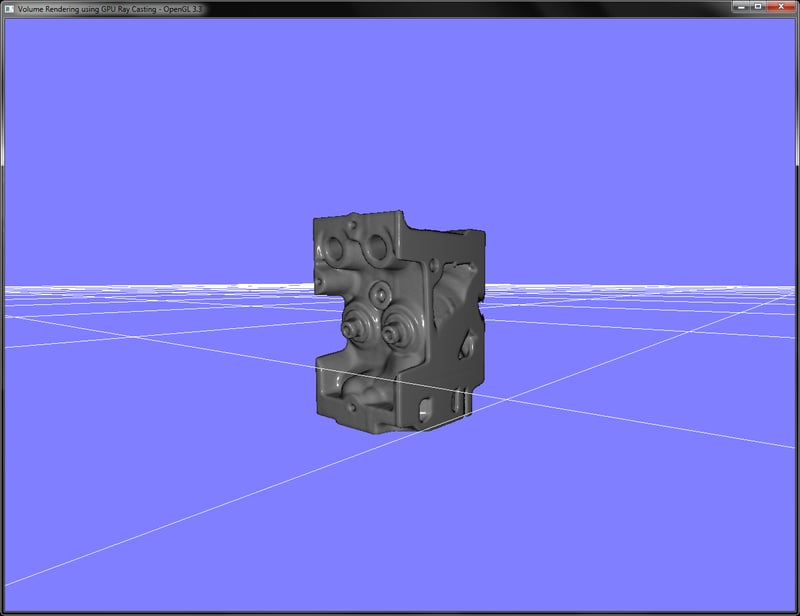
We will now implement pseudo-isosurface rendering in single-pass GPU ray casting. While much of the setup is the same as for the single-pass GPU ray casting, the difference will be in the compositing step in the ray casting fragment shader. In this shader, we will try to find the given isosurface. If it is actually found, we estimate the normal at the sampling point to carry out the lighting calculation for the isosurface.
The code for this recipe is in the Chapter7/GPURaycastingIsosurface folder. We will be starting from the single-pass GPU ray casting recipe using the exact same application side code.
Let us start the recipe by following these simple steps:
- Load the volume data from file into a 3D OpenGL texture as in the previous recipe. Refer to the
LoadVolumefunction inChapter7/GPURaycasting/main.cppfor details. - Set up a vertex array object and a vertex buffer object to render a unit cube as in the previous recipe.
- In the render function, set the ray casting vertex and fragment shaders (
Chapter7/GPURaycasting/shaders/raycasting(vert,frag)) and then render the unit cube.glEnable(GL_BLEND); glBindVertexArray(cubeVAOID); shader.Use(); glUniformMatrix4fv(shader("MVP"), 1, GL_FALSE, glm::value_ptr(MVP)); glUniform3fv(shader("camPos"), 1, &(camPos.x)); glDrawElements(GL_TRIANGLES, 36, GL_UNSIGNED_SHORT, 0); shader.UnUse(); glDisable(GL_BLEND); - From the vertex shader, in addition to the clip-space position, output the 3D texture coordinates for lookup in the fragment shader. We simply offset the object space vertex positions as follows:
smooth out vec3 vUV; void main() { gl_Position = MVP*vec4(vVertex.xyz,1); vUV = vVertex + vec3(0.5); } - In the fragment shader, use the camera position and the 3D texture coordinates to run a loop in the current viewing direction. The loop is terminated if the current sample position is outside the volume or the alpha value of the accumulated color is saturated.
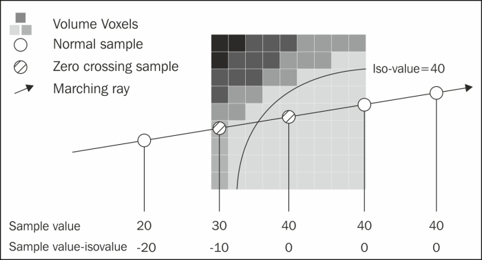
vec3 dataPos = vUV; vec3 geomDir = normalize((vUV-vec3(0.5)) - camPos); vec3 dirStep = geomDir * step_size; bool stop = false; for (int i = 0; i < MAX_SAMPLES; i++) { // advance ray by step dataPos = dataPos + dirStep; // stop condition stop=dot(sign(dataPos-texMin),sign(texMax-dataPos)) < 3.0; if (stop) break; - For isosurface estimation, we take two sample values to find the zero crossing of the isofunction inside the volume dataset. If there is a zero crossing, we find the exact intersection point using bisection based refinement. Finally, we use the Phong illumination model to shade the isosurface assuming that the light is located at the camera position.
float sample=texture(volume, dataPos).r; float sample2=texture(volume, dataPos+dirStep).r; if( (sample -isoValue) < 0 && (sample2-isoValue) >= 0.0){ vec3 xN = dataPos; vec3 xF = dataPos+dirStep; vec3 tc = Bisection(xN, xF, isoValue); vec3 N = GetGradient(tc); vec3 V = -geomDir; vec3 L = V; vFragColor = PhongLighting(L,N,V,250, vec3(0.5)); break; } }
The Bisection function is defined as follows:
The Bisection function takes the two samples between which the given sample value lies. It then runs a loop. In each step, it calculates the midpoint of the two sample points and checks the density value at the midpoint to the given isovalue. If it is less, the left sample point is swapped with the mid position otherwise, the right sample point is swapped. This helps to reduce the search space quickly. The process is repeated and finally, the midpoint between the left sample point and right sample point is returned. The Gradient function estimates the gradient of the volume density using center finite difference approximation.
While bulk of the code is similar to the single-pass GPU ray casting recipe. There is a major difference in the ray marching loop. In case of isosurface rendering, we do not use compositing. Instead, we find the zero crossing of the volume dataset isofunction by sampling two consecutive samples. This is well illustrated with the following diagram. If there is a zero crossing, we refine the detected isosurface by using bisection-based refinement.
recipe is in the Chapter7/GPURaycastingIsosurface folder. We will be starting from the single-pass GPU ray casting recipe using the exact same application side code.
Let us start the recipe by following these simple steps:
- Load the volume data from file into a 3D OpenGL texture as in the previous recipe. Refer to the
LoadVolumefunction inChapter7/GPURaycasting/main.cppfor details. - Set up a vertex array object and a vertex buffer object to render a unit cube as in the previous recipe.
- In the render function, set the ray casting vertex and fragment shaders (
Chapter7/GPURaycasting/shaders/raycasting(vert,frag)) and then render the unit cube.glEnable(GL_BLEND); glBindVertexArray(cubeVAOID); shader.Use(); glUniformMatrix4fv(shader("MVP"), 1, GL_FALSE, glm::value_ptr(MVP)); glUniform3fv(shader("camPos"), 1, &(camPos.x)); glDrawElements(GL_TRIANGLES, 36, GL_UNSIGNED_SHORT, 0); shader.UnUse(); glDisable(GL_BLEND); - From the vertex shader, in addition to the clip-space position, output the 3D texture coordinates for lookup in the fragment shader. We simply offset the object space vertex positions as follows:
smooth out vec3 vUV; void main() { gl_Position = MVP*vec4(vVertex.xyz,1); vUV = vVertex + vec3(0.5); } - In the fragment shader, use the camera position and the 3D texture coordinates to run a loop in the current viewing direction. The loop is terminated if the current sample position is outside the volume or the alpha value of the accumulated color is saturated.
vec3 dataPos = vUV; vec3 geomDir = normalize((vUV-vec3(0.5)) - camPos); vec3 dirStep = geomDir * step_size; bool stop = false; for (int i = 0; i < MAX_SAMPLES; i++) { // advance ray by step dataPos = dataPos + dirStep; // stop condition stop=dot(sign(dataPos-texMin),sign(texMax-dataPos)) < 3.0; if (stop) break; - For isosurface estimation, we take two sample values to find the zero crossing of the isofunction inside the volume dataset. If there is a zero crossing, we find the exact intersection point using bisection based refinement. Finally, we use the Phong illumination model to shade the isosurface assuming that the light is located at the camera position.
float sample=texture(volume, dataPos).r; float sample2=texture(volume, dataPos+dirStep).r; if( (sample -isoValue) < 0 && (sample2-isoValue) >= 0.0){ vec3 xN = dataPos; vec3 xF = dataPos+dirStep; vec3 tc = Bisection(xN, xF, isoValue); vec3 N = GetGradient(tc); vec3 V = -geomDir; vec3 L = V; vFragColor = PhongLighting(L,N,V,250, vec3(0.5)); break; } }
The Bisection function is defined as follows:
The Bisection function takes the two samples between which the given sample value lies. It then runs a loop. In each step, it calculates the midpoint of the two sample points and checks the density value at the midpoint to the given isovalue. If it is less, the left sample point is swapped with the mid position otherwise, the right sample point is swapped. This helps to reduce the search space quickly. The process is repeated and finally, the midpoint between the left sample point and right sample point is returned. The Gradient function estimates the gradient of the volume density using center finite difference approximation.
While bulk of the code is similar to the single-pass GPU ray casting recipe. There is a major difference in the ray marching loop. In case of isosurface rendering, we do not use compositing. Instead, we find the zero crossing of the volume dataset isofunction by sampling two consecutive samples. This is well illustrated with the following diagram. If there is a zero crossing, we refine the detected isosurface by using bisection-based refinement.
LoadVolume function in Chapter7/GPURaycasting/main.cpp for details.
Chapter7/GPURaycasting/shaders/raycasting (vert,frag)) and then render the unit cube.glEnable(GL_BLEND);
glBindVertexArray(cubeVAOID);
shader.Use();
glUniformMatrix4fv(shader("MVP"), 1, GL_FALSE, glm::value_ptr(MVP));
glUniform3fv(shader("camPos"), 1, &(camPos.x));
glDrawElements(GL_TRIANGLES, 36, GL_UNSIGNED_SHORT, 0);
shader.UnUse();
glDisable(GL_BLEND);smooth out vec3 vUV;
void main()
{
gl_Position = MVP*vec4(vVertex.xyz,1);
vUV = vVertex + vec3(0.5);
}- shader, use the camera position and the 3D texture coordinates to run a loop in the current viewing direction. The loop is terminated if the current sample position is outside the volume or the alpha value of the accumulated color is saturated.
vec3 dataPos = vUV; vec3 geomDir = normalize((vUV-vec3(0.5)) - camPos); vec3 dirStep = geomDir * step_size; bool stop = false; for (int i = 0; i < MAX_SAMPLES; i++) { // advance ray by step dataPos = dataPos + dirStep; // stop condition stop=dot(sign(dataPos-texMin),sign(texMax-dataPos)) < 3.0; if (stop) break; - For isosurface estimation, we take two sample values to find the zero crossing of the isofunction inside the volume dataset. If there is a zero crossing, we find the exact intersection point using bisection based refinement. Finally, we use the Phong illumination model to shade the isosurface assuming that the light is located at the camera position.
float sample=texture(volume, dataPos).r; float sample2=texture(volume, dataPos+dirStep).r; if( (sample -isoValue) < 0 && (sample2-isoValue) >= 0.0){ vec3 xN = dataPos; vec3 xF = dataPos+dirStep; vec3 tc = Bisection(xN, xF, isoValue); vec3 N = GetGradient(tc); vec3 V = -geomDir; vec3 L = V; vFragColor = PhongLighting(L,N,V,250, vec3(0.5)); break; } }
The Bisection function is defined as follows:
The Bisection function takes the two samples between which the given sample value lies. It then runs a loop. In each step, it calculates the midpoint of the two sample points and checks the density value at the midpoint to the given isovalue. If it is less, the left sample point is swapped with the mid position otherwise, the right sample point is swapped. This helps to reduce the search space quickly. The process is repeated and finally, the midpoint between the left sample point and right sample point is returned. The Gradient function estimates the gradient of the volume density using center finite difference approximation.
While bulk of the code is similar to the single-pass GPU ray casting recipe. There is a major difference in the ray marching loop. In case of isosurface rendering, we do not use compositing. Instead, we find the zero crossing of the volume dataset isofunction by sampling two consecutive samples. This is well illustrated with the following diagram. If there is a zero crossing, we refine the detected isosurface by using bisection-based refinement.
samples. This is well illustrated with the following diagram. If there is a zero crossing, we refine the detected isosurface by using bisection-based refinement.
In this recipe, we will implement splatting on the GPU. The splatting algorithm converts the voxel representation into splats by convolving them with a Gaussian kernel. The Gaussian smoothing kernel reduces high frequencies and smoothes out edges giving a smoothed rendered output.
Let us start this recipe by following these simple steps:
- Load the 3D volume data and store it into an array.
std::ifstream infile(filename.c_str(), std::ios_base::binary); if(infile.good()) { pVolume = new GLubyte[XDIM*YDIM*ZDIM]; infile.read(reinterpret_cast<char*>(pVolume), XDIM*YDIM*ZDIM*sizeof(GLubyte)); infile.close(); return true; } else { return false; } - Depending on the sampling box size, run three loops to iterate through the entire volume voxel by voxel.
vertices.clear(); int dx = XDIM/X_SAMPLING_DIST; int dy = YDIM/Y_SAMPLING_DIST; int dz = ZDIM/Z_SAMPLING_DIST; scale = glm::vec3(dx,dy,dz); for(int z=0;z<ZDIM;z+=dz) { for(int y=0;y<YDIM;y+=dy) { for(int x=0;x<XDIM;x+=dx) { SampleVoxel(x,y,z); } } }The
SampleVoxelfunction is defined in theVolumeSplatterclass as follows: - In each sampling step, estimate the volume density values at the current voxel. If the value is greater than the given isovalue, store the voxel position and normal into a vertex array.
GLubyte data = SampleVolume(x, y, z); if(data>isoValue) { Vertex v; v.pos.x = x; v.pos.y = y; v.pos.z = z; v.normal = GetNormal(x, y, z); v.pos *= invDim; vertices.push_back(v); }The
SampleVolumefunction takes the given sampling point and returns the nearest voxel density. It is defined in theVolumeSplatterclass as follows:GLubyte VolumeSplatter::SampleVolume(const int x, const int y, const int z) { int index = (x+(y*XDIM)) + z*(XDIM*YDIM); if(index<0) index = 0; if(index >= XDIM*YDIM*ZDIM) index = (XDIM*YDIM*ZDIM)-1; return pVolume[index]; } - After the sampling step, pass the generated vertices to a vertex array object (VAO) containing a vertex buffer object (VBO).
glGenVertexArrays(1, &volumeSplatterVAO); glGenBuffers(1, &volumeSplatterVBO); glBindVertexArray(volumeSplatterVAO); glBindBuffer (GL_ARRAY_BUFFER, volumeSplatterVBO); glBufferData (GL_ARRAY_BUFFER, splatter->GetTotalVertices() *sizeof(Vertex), splatter->GetVertexPointer(), GL_STATIC_DRAW); glEnableVertexAttribArray(0); glVertexAttribPointer(0, 3, GL_FLOAT, GL_FALSE,sizeof(Vertex), 0); glEnableVertexAttribArray(1); glVertexAttribPointer(1, 3, GL_FLOAT, GL_FALSE,sizeof(Vertex), (const GLvoid*) offsetof(Vertex, normal));
- Set up two FBOs for offscreen rendering. The first FBO (
filterFBOID) is used for Gaussian smoothing.glGenFramebuffers(1,&filterFBOID); glBindFramebuffer(GL_FRAMEBUFFER,filterFBOID); glGenTextures(2, blurTexID); for(int i=0;i<2;i++) { glActiveTexture(GL_TEXTURE1+i); glBindTexture(GL_TEXTURE_2D, blurTexID[i]); //set texture parameters glTexImage2D(GL_TEXTURE_2D,0,GL_RGBA32F,IMAGE_WIDTH, IMAGE_HEIGHT,0,GL_RGBA,GL_FLOAT,NULL); glFramebufferTexture2D(GL_FRAMEBUFFER, GL_COLOR_ATTACHMENT0+i,GL_TEXTURE_2D,blurTexID[i],0); } GLenum status = glCheckFramebufferStatus(GL_FRAMEBUFFER); if(status == GL_FRAMEBUFFER_COMPLETE) { cout<<"Filtering FBO setup successful."<<endl; } else { cout<<"Problem in Filtering FBO setup."<<endl; } - The second FBO (
fboID) is used to render the scene so that the smoothing operation can be applied on the rendered output from the first pass. Add a render buffer object to this FBO to enable depth testing.glGenFramebuffers(1,&fboID); glGenRenderbuffers(1, &rboID); glGenTextures(1, &texID); glBindFramebuffer(GL_FRAMEBUFFER,fboID); glBindRenderbuffer(GL_RENDERBUFFER, rboID); glActiveTexture(GL_TEXTURE0); glBindTexture(GL_TEXTURE_2D, texID); //set texture parameters glTexImage2D(GL_TEXTURE_2D,0,GL_RGBA32F,IMAGE_WIDTH, IMAGE_HEIGHT,0,GL_RGBA,GL_FLOAT,NULL); glFramebufferTexture2D(GL_FRAMEBUFFER,GL_COLOR_ATTACHMENT0, GL_TEXTURE_2D, texID, 0); glFramebufferRenderbuffer(GL_FRAMEBUFFER, GL_DEPTH_ATTACHMENT, GL_RENDERBUFFER, rboID); glRenderbufferStorage(GL_RENDERBUFFER, GL_DEPTH_COMPONENT32, IMAGE_WIDTH, IMAGE_HEIGHT); status = glCheckFramebufferStatus(GL_FRAMEBUFFER); if(status == GL_FRAMEBUFFER_COMPLETE) { cout<<"Offscreen rendering FBO setup successful."<<endl; } else { cout<<"Problem in offscreen rendering FBO setup."<<endl; }
- In the render function, first render the point splats to a texture using the first FBO (
fboID).glBindFramebuffer(GL_FRAMEBUFFER,fboID); glViewport(0,0, IMAGE_WIDTH, IMAGE_HEIGHT); glDrawBuffer(GL_COLOR_ATTACHMENT0); glClear(GL_COLOR_BUFFER_BIT|GL_DEPTH_BUFFER_BIT); glm::mat4 T = glm::translate(glm::mat4(1), glm::vec3(-0.5,-0.5,-0.5)); glBindVertexArray(volumeSplatterVAO); shader.Use(); glUniformMatrix4fv(shader("MV"), 1, GL_FALSE, glm::value_ptr(MV*T)); glUniformMatrix3fv(shader("N"), 1, GL_FALSE, glm::value_ptr(glm::inverseTranspose(glm::mat3(MV*T)))); glUniformMatrix4fv(shader("P"), 1, GL_FALSE, glm::value_ptr(P)); glDrawArrays(GL_POINTS, 0, splatter->GetTotalVertices()); shader.UnUse();The splatting vertex shader (
Chapter7/Splatting/shaders/splatShader.vert) is defined as follows. It calculates the eye space normal. The splat size is calculated using the volume dimension and the sampling voxel size. This is then written to thegl_PointSizevariable in the vertex shader.The splatting fragment shader (
Chapter7/Splatting/shaders/splatShader.frag) is defined as follows: - Next, set the filtering FBO and first apply the vertical and then the horizontal Gaussian smoothing pass by drawing a full-screen quad as was done in the Variance shadow mapping recipe in Chapter 4, Lights and Shadows.
glBindVertexArray(quadVAOID); glBindFramebuffer(GL_FRAMEBUFFER, filterFBOID); glDrawBuffer(GL_COLOR_ATTACHMENT0); gaussianV_shader.Use(); glDrawElements(GL_TRIANGLES, 6, GL_UNSIGNED_SHORT, 0); glDrawBuffer(GL_COLOR_ATTACHMENT1); gaussianH_shader.Use(); glDrawElements(GL_TRIANGLES, 6, GL_UNSIGNED_SHORT, 0);
- Unbind the filtering FBO, restore the default draw buffer and render the filtered output on the screen.
glBindFramebuffer(GL_FRAMEBUFFER,0); glDrawBuffer(GL_BACK_LEFT); glViewport(0,0,WIDTH, HEIGHT); quadShader.Use(); glDrawElements(GL_TRIANGLES, 6, GL_UNSIGNED_SHORT, 0); quadShader.UnUse(); glBindVertexArray(0);
Splatting algorithm works by rendering the voxels of the volume data as Gaussian blobs and projecting them on the screen. To achieve this, we first estimate the candidate voxels from the volume dataset by traversing through the entire volume dataset voxel by voxel for the given isovalue. If we have the appropriate voxel, we store its normal and position into a vertex array. For convenience, we wrap all of this functionality into the VolumeSplatter class.
Finally, we estimate the diffuse and specular components and output the current fragment color using the eye space normal of the splat.
This recipe gave us an overview on the splatting algorithm. Our brute force approach in this recipe was to iterate through all of the voxels. For large datasets, we have to employ an acceleration structure, like an octree, to quickly identify voxels with densities and cull unnecessary voxels.
- The Qsplat project: http://graphics.stanford.edu/software/qsplat/
- Splatting research at ETH Zurich: (http://graphics.ethz.ch/research/past_projects/surfels/surfacesplatting/)
Chapter7/Splatting directory.
Let us start this recipe by following these simple steps:
- Load the 3D volume data and store it into an array.
std::ifstream infile(filename.c_str(), std::ios_base::binary); if(infile.good()) { pVolume = new GLubyte[XDIM*YDIM*ZDIM]; infile.read(reinterpret_cast<char*>(pVolume), XDIM*YDIM*ZDIM*sizeof(GLubyte)); infile.close(); return true; } else { return false; } - Depending on the sampling box size, run three loops to iterate through the entire volume voxel by voxel.
vertices.clear(); int dx = XDIM/X_SAMPLING_DIST; int dy = YDIM/Y_SAMPLING_DIST; int dz = ZDIM/Z_SAMPLING_DIST; scale = glm::vec3(dx,dy,dz); for(int z=0;z<ZDIM;z+=dz) { for(int y=0;y<YDIM;y+=dy) { for(int x=0;x<XDIM;x+=dx) { SampleVoxel(x,y,z); } } }The
SampleVoxelfunction is defined in theVolumeSplatterclass as follows: - In each sampling step, estimate the volume density values at the current voxel. If the value is greater than the given isovalue, store the voxel position and normal into a vertex array.
GLubyte data = SampleVolume(x, y, z); if(data>isoValue) { Vertex v; v.pos.x = x; v.pos.y = y; v.pos.z = z; v.normal = GetNormal(x, y, z); v.pos *= invDim; vertices.push_back(v); }The
SampleVolumefunction takes the given sampling point and returns the nearest voxel density. It is defined in theVolumeSplatterclass as follows:GLubyte VolumeSplatter::SampleVolume(const int x, const int y, const int z) { int index = (x+(y*XDIM)) + z*(XDIM*YDIM); if(index<0) index = 0; if(index >= XDIM*YDIM*ZDIM) index = (XDIM*YDIM*ZDIM)-1; return pVolume[index]; } - After the sampling step, pass the generated vertices to a vertex array object (VAO) containing a vertex buffer object (VBO).
glGenVertexArrays(1, &volumeSplatterVAO); glGenBuffers(1, &volumeSplatterVBO); glBindVertexArray(volumeSplatterVAO); glBindBuffer (GL_ARRAY_BUFFER, volumeSplatterVBO); glBufferData (GL_ARRAY_BUFFER, splatter->GetTotalVertices() *sizeof(Vertex), splatter->GetVertexPointer(), GL_STATIC_DRAW); glEnableVertexAttribArray(0); glVertexAttribPointer(0, 3, GL_FLOAT, GL_FALSE,sizeof(Vertex), 0); glEnableVertexAttribArray(1); glVertexAttribPointer(1, 3, GL_FLOAT, GL_FALSE,sizeof(Vertex), (const GLvoid*) offsetof(Vertex, normal));
- Set up two FBOs for offscreen rendering. The first FBO (
filterFBOID) is used for Gaussian smoothing.glGenFramebuffers(1,&filterFBOID); glBindFramebuffer(GL_FRAMEBUFFER,filterFBOID); glGenTextures(2, blurTexID); for(int i=0;i<2;i++) { glActiveTexture(GL_TEXTURE1+i); glBindTexture(GL_TEXTURE_2D, blurTexID[i]); //set texture parameters glTexImage2D(GL_TEXTURE_2D,0,GL_RGBA32F,IMAGE_WIDTH, IMAGE_HEIGHT,0,GL_RGBA,GL_FLOAT,NULL); glFramebufferTexture2D(GL_FRAMEBUFFER, GL_COLOR_ATTACHMENT0+i,GL_TEXTURE_2D,blurTexID[i],0); } GLenum status = glCheckFramebufferStatus(GL_FRAMEBUFFER); if(status == GL_FRAMEBUFFER_COMPLETE) { cout<<"Filtering FBO setup successful."<<endl; } else { cout<<"Problem in Filtering FBO setup."<<endl; } - The second FBO (
fboID) is used to render the scene so that the smoothing operation can be applied on the rendered output from the first pass. Add a render buffer object to this FBO to enable depth testing.glGenFramebuffers(1,&fboID); glGenRenderbuffers(1, &rboID); glGenTextures(1, &texID); glBindFramebuffer(GL_FRAMEBUFFER,fboID); glBindRenderbuffer(GL_RENDERBUFFER, rboID); glActiveTexture(GL_TEXTURE0); glBindTexture(GL_TEXTURE_2D, texID); //set texture parameters glTexImage2D(GL_TEXTURE_2D,0,GL_RGBA32F,IMAGE_WIDTH, IMAGE_HEIGHT,0,GL_RGBA,GL_FLOAT,NULL); glFramebufferTexture2D(GL_FRAMEBUFFER,GL_COLOR_ATTACHMENT0, GL_TEXTURE_2D, texID, 0); glFramebufferRenderbuffer(GL_FRAMEBUFFER, GL_DEPTH_ATTACHMENT, GL_RENDERBUFFER, rboID); glRenderbufferStorage(GL_RENDERBUFFER, GL_DEPTH_COMPONENT32, IMAGE_WIDTH, IMAGE_HEIGHT); status = glCheckFramebufferStatus(GL_FRAMEBUFFER); if(status == GL_FRAMEBUFFER_COMPLETE) { cout<<"Offscreen rendering FBO setup successful."<<endl; } else { cout<<"Problem in offscreen rendering FBO setup."<<endl; }
- In the render function, first render the point splats to a texture using the first FBO (
fboID).glBindFramebuffer(GL_FRAMEBUFFER,fboID); glViewport(0,0, IMAGE_WIDTH, IMAGE_HEIGHT); glDrawBuffer(GL_COLOR_ATTACHMENT0); glClear(GL_COLOR_BUFFER_BIT|GL_DEPTH_BUFFER_BIT); glm::mat4 T = glm::translate(glm::mat4(1), glm::vec3(-0.5,-0.5,-0.5)); glBindVertexArray(volumeSplatterVAO); shader.Use(); glUniformMatrix4fv(shader("MV"), 1, GL_FALSE, glm::value_ptr(MV*T)); glUniformMatrix3fv(shader("N"), 1, GL_FALSE, glm::value_ptr(glm::inverseTranspose(glm::mat3(MV*T)))); glUniformMatrix4fv(shader("P"), 1, GL_FALSE, glm::value_ptr(P)); glDrawArrays(GL_POINTS, 0, splatter->GetTotalVertices()); shader.UnUse();The splatting vertex shader (
Chapter7/Splatting/shaders/splatShader.vert) is defined as follows. It calculates the eye space normal. The splat size is calculated using the volume dimension and the sampling voxel size. This is then written to thegl_PointSizevariable in the vertex shader.The splatting fragment shader (
Chapter7/Splatting/shaders/splatShader.frag) is defined as follows: - Next, set the filtering FBO and first apply the vertical and then the horizontal Gaussian smoothing pass by drawing a full-screen quad as was done in the Variance shadow mapping recipe in Chapter 4, Lights and Shadows.
glBindVertexArray(quadVAOID); glBindFramebuffer(GL_FRAMEBUFFER, filterFBOID); glDrawBuffer(GL_COLOR_ATTACHMENT0); gaussianV_shader.Use(); glDrawElements(GL_TRIANGLES, 6, GL_UNSIGNED_SHORT, 0); glDrawBuffer(GL_COLOR_ATTACHMENT1); gaussianH_shader.Use(); glDrawElements(GL_TRIANGLES, 6, GL_UNSIGNED_SHORT, 0);
- Unbind the filtering FBO, restore the default draw buffer and render the filtered output on the screen.
glBindFramebuffer(GL_FRAMEBUFFER,0); glDrawBuffer(GL_BACK_LEFT); glViewport(0,0,WIDTH, HEIGHT); quadShader.Use(); glDrawElements(GL_TRIANGLES, 6, GL_UNSIGNED_SHORT, 0); quadShader.UnUse(); glBindVertexArray(0);
Splatting algorithm works by rendering the voxels of the volume data as Gaussian blobs and projecting them on the screen. To achieve this, we first estimate the candidate voxels from the volume dataset by traversing through the entire volume dataset voxel by voxel for the given isovalue. If we have the appropriate voxel, we store its normal and position into a vertex array. For convenience, we wrap all of this functionality into the VolumeSplatter class.
Finally, we estimate the diffuse and specular components and output the current fragment color using the eye space normal of the splat.
This recipe gave us an overview on the splatting algorithm. Our brute force approach in this recipe was to iterate through all of the voxels. For large datasets, we have to employ an acceleration structure, like an octree, to quickly identify voxels with densities and cull unnecessary voxels.
- The Qsplat project: http://graphics.stanford.edu/software/qsplat/
- Splatting research at ETH Zurich: (http://graphics.ethz.ch/research/past_projects/surfels/surfacesplatting/)
std::ifstream infile(filename.c_str(), std::ios_base::binary);
if(infile.good()) {
pVolume = new GLubyte[XDIM*YDIM*ZDIM];
infile.read(reinterpret_cast<char*>(pVolume), XDIM*YDIM*ZDIM*sizeof(GLubyte));
infile.close();
return true;
} else {
return false;
}vertices.clear();
int dx = XDIM/X_SAMPLING_DIST;
int dy = YDIM/Y_SAMPLING_DIST;
int dz = ZDIM/Z_SAMPLING_DIST;
scale = glm::vec3(dx,dy,dz);
for(int z=0;z<ZDIM;z+=dz) {
for(int y=0;y<YDIM;y+=dy) {
for(int x=0;x<XDIM;x+=dx) {
SampleVoxel(x,y,z);
}
}
}SampleVoxel function
- In each sampling step, estimate the volume density values at the current voxel. If the value is greater than the given isovalue, store the voxel position and normal into a vertex array.
GLubyte data = SampleVolume(x, y, z); if(data>isoValue) { Vertex v; v.pos.x = x; v.pos.y = y; v.pos.z = z; v.normal = GetNormal(x, y, z); v.pos *= invDim; vertices.push_back(v); }The
SampleVolumefunction takes the given sampling point and returns the nearest voxel density. It is defined in theVolumeSplatterclass as follows:GLubyte VolumeSplatter::SampleVolume(const int x, const int y, const int z) { int index = (x+(y*XDIM)) + z*(XDIM*YDIM); if(index<0) index = 0; if(index >= XDIM*YDIM*ZDIM) index = (XDIM*YDIM*ZDIM)-1; return pVolume[index]; } - After the sampling step, pass the generated vertices to a vertex array object (VAO) containing a vertex buffer object (VBO).
glGenVertexArrays(1, &volumeSplatterVAO); glGenBuffers(1, &volumeSplatterVBO); glBindVertexArray(volumeSplatterVAO); glBindBuffer (GL_ARRAY_BUFFER, volumeSplatterVBO); glBufferData (GL_ARRAY_BUFFER, splatter->GetTotalVertices() *sizeof(Vertex), splatter->GetVertexPointer(), GL_STATIC_DRAW); glEnableVertexAttribArray(0); glVertexAttribPointer(0, 3, GL_FLOAT, GL_FALSE,sizeof(Vertex), 0); glEnableVertexAttribArray(1); glVertexAttribPointer(1, 3, GL_FLOAT, GL_FALSE,sizeof(Vertex), (const GLvoid*) offsetof(Vertex, normal));
- Set up two FBOs for offscreen rendering. The first FBO (
filterFBOID) is used for Gaussian smoothing.glGenFramebuffers(1,&filterFBOID); glBindFramebuffer(GL_FRAMEBUFFER,filterFBOID); glGenTextures(2, blurTexID); for(int i=0;i<2;i++) { glActiveTexture(GL_TEXTURE1+i); glBindTexture(GL_TEXTURE_2D, blurTexID[i]); //set texture parameters glTexImage2D(GL_TEXTURE_2D,0,GL_RGBA32F,IMAGE_WIDTH, IMAGE_HEIGHT,0,GL_RGBA,GL_FLOAT,NULL); glFramebufferTexture2D(GL_FRAMEBUFFER, GL_COLOR_ATTACHMENT0+i,GL_TEXTURE_2D,blurTexID[i],0); } GLenum status = glCheckFramebufferStatus(GL_FRAMEBUFFER); if(status == GL_FRAMEBUFFER_COMPLETE) { cout<<"Filtering FBO setup successful."<<endl; } else { cout<<"Problem in Filtering FBO setup."<<endl; } - The second FBO (
fboID) is used to render the scene so that the smoothing operation can be applied on the rendered output from the first pass. Add a render buffer object to this FBO to enable depth testing.glGenFramebuffers(1,&fboID); glGenRenderbuffers(1, &rboID); glGenTextures(1, &texID); glBindFramebuffer(GL_FRAMEBUFFER,fboID); glBindRenderbuffer(GL_RENDERBUFFER, rboID); glActiveTexture(GL_TEXTURE0); glBindTexture(GL_TEXTURE_2D, texID); //set texture parameters glTexImage2D(GL_TEXTURE_2D,0,GL_RGBA32F,IMAGE_WIDTH, IMAGE_HEIGHT,0,GL_RGBA,GL_FLOAT,NULL); glFramebufferTexture2D(GL_FRAMEBUFFER,GL_COLOR_ATTACHMENT0, GL_TEXTURE_2D, texID, 0); glFramebufferRenderbuffer(GL_FRAMEBUFFER, GL_DEPTH_ATTACHMENT, GL_RENDERBUFFER, rboID); glRenderbufferStorage(GL_RENDERBUFFER, GL_DEPTH_COMPONENT32, IMAGE_WIDTH, IMAGE_HEIGHT); status = glCheckFramebufferStatus(GL_FRAMEBUFFER); if(status == GL_FRAMEBUFFER_COMPLETE) { cout<<"Offscreen rendering FBO setup successful."<<endl; } else { cout<<"Problem in offscreen rendering FBO setup."<<endl; }
- In the render function, first render the point splats to a texture using the first FBO (
fboID).glBindFramebuffer(GL_FRAMEBUFFER,fboID); glViewport(0,0, IMAGE_WIDTH, IMAGE_HEIGHT); glDrawBuffer(GL_COLOR_ATTACHMENT0); glClear(GL_COLOR_BUFFER_BIT|GL_DEPTH_BUFFER_BIT); glm::mat4 T = glm::translate(glm::mat4(1), glm::vec3(-0.5,-0.5,-0.5)); glBindVertexArray(volumeSplatterVAO); shader.Use(); glUniformMatrix4fv(shader("MV"), 1, GL_FALSE, glm::value_ptr(MV*T)); glUniformMatrix3fv(shader("N"), 1, GL_FALSE, glm::value_ptr(glm::inverseTranspose(glm::mat3(MV*T)))); glUniformMatrix4fv(shader("P"), 1, GL_FALSE, glm::value_ptr(P)); glDrawArrays(GL_POINTS, 0, splatter->GetTotalVertices()); shader.UnUse();The splatting vertex shader (
Chapter7/Splatting/shaders/splatShader.vert) is defined as follows. It calculates the eye space normal. The splat size is calculated using the volume dimension and the sampling voxel size. This is then written to thegl_PointSizevariable in the vertex shader.The splatting fragment shader (
Chapter7/Splatting/shaders/splatShader.frag) is defined as follows: - Next, set the filtering FBO and first apply the vertical and then the horizontal Gaussian smoothing pass by drawing a full-screen quad as was done in the Variance shadow mapping recipe in Chapter 4, Lights and Shadows.
glBindVertexArray(quadVAOID); glBindFramebuffer(GL_FRAMEBUFFER, filterFBOID); glDrawBuffer(GL_COLOR_ATTACHMENT0); gaussianV_shader.Use(); glDrawElements(GL_TRIANGLES, 6, GL_UNSIGNED_SHORT, 0); glDrawBuffer(GL_COLOR_ATTACHMENT1); gaussianH_shader.Use(); glDrawElements(GL_TRIANGLES, 6, GL_UNSIGNED_SHORT, 0);
- Unbind the filtering FBO, restore the default draw buffer and render the filtered output on the screen.
glBindFramebuffer(GL_FRAMEBUFFER,0); glDrawBuffer(GL_BACK_LEFT); glViewport(0,0,WIDTH, HEIGHT); quadShader.Use(); glDrawElements(GL_TRIANGLES, 6, GL_UNSIGNED_SHORT, 0); quadShader.UnUse(); glBindVertexArray(0);
Splatting algorithm works by rendering the voxels of the volume data as Gaussian blobs and projecting them on the screen. To achieve this, we first estimate the candidate voxels from the volume dataset by traversing through the entire volume dataset voxel by voxel for the given isovalue. If we have the appropriate voxel, we store its normal and position into a vertex array. For convenience, we wrap all of this functionality into the VolumeSplatter class.
Finally, we estimate the diffuse and specular components and output the current fragment color using the eye space normal of the splat.
This recipe gave us an overview on the splatting algorithm. Our brute force approach in this recipe was to iterate through all of the voxels. For large datasets, we have to employ an acceleration structure, like an octree, to quickly identify voxels with densities and cull unnecessary voxels.
- The Qsplat project: http://graphics.stanford.edu/software/qsplat/
- Splatting research at ETH Zurich: (http://graphics.ethz.ch/research/past_projects/surfels/surfacesplatting/)
algorithm works by rendering the voxels of the volume data as Gaussian blobs and projecting them on the screen. To achieve this, we first estimate the candidate voxels from the volume dataset by traversing through the entire volume dataset voxel by voxel for the given isovalue. If we have the appropriate voxel, we store its normal and position into a vertex array. For convenience, we wrap all of this functionality into the VolumeSplatter class.
Finally, we estimate the diffuse and specular components and output the current fragment color using the eye space normal of the splat.
This recipe gave us an overview on the splatting algorithm. Our brute force approach in this recipe was to iterate through all of the voxels. For large datasets, we have to employ an acceleration structure, like an octree, to quickly identify voxels with densities and cull unnecessary voxels.
- The Qsplat project: http://graphics.stanford.edu/software/qsplat/
- Splatting research at ETH Zurich: (http://graphics.ethz.ch/research/past_projects/surfels/surfacesplatting/)
acceleration structure, like an octree, to quickly identify voxels with densities and cull unnecessary voxels.
- The Qsplat project: http://graphics.stanford.edu/software/qsplat/
- Splatting research at ETH Zurich: (http://graphics.ethz.ch/research/past_projects/surfels/surfacesplatting/)
- http://graphics.stanford.edu/software/qsplat/
- Splatting research at ETH Zurich: (http://graphics.ethz.ch/research/past_projects/surfels/surfacesplatting/)
In this recipe, we will implement classification to the 3D texture slicing presented before. We will generate a lookup table to add specific colors to specific densities. This is accomplished by generating a 1D texture that is looked up in the fragment shader with the current volume density. The returned color is then used as the color of the current fragment. Apart from the setup of the transfer function data, all the other content remains the same as in the 3D texture slicing recipe. Note that the classification method is not limited to 3D texture slicing, it can be applied to any volume rendering algorithm.
Let us start this recipe by following these simple steps:
- Load the volume data and setup the texture slicing as in the Implementing volume rendering using 3D texture slicing recipe.
- Create a 1D texture that will be our transfer function texture for color lookup. We create a set of color values and then interpolate them on the fly. Refer to
LoadTransferFunctioninChapter7/3DTextureSlicingClassification/main.cpp.float pData[256][4]; int indices[9]; for(int i=0;i<9;i++) { int index = i*28; pData[index][0] = jet_values[i].x; pData[index][1] = jet_values[i].y; pData[index][2] = jet_values[i].z; pData[index][3] = jet_values[i].w; indices[i] = index; } for(int j=0;j<9-1;j++) { float dDataR = (pData[indices[j+1]][0] - pData[indices[j]][0]); float dDataG = (pData[indices[j+1]][1] - pData[indices[j]][1]); float dDataB = (pData[indices[j+1]][2] - pData[indices[j]][2]); float dDataA = (pData[indices[j+1]][3] - pData[indices[j]][3]); int dIndex = indices[j+1]-indices[j]; float dDataIncR = dDataR/float(dIndex); float dDataIncG = dDataG/float(dIndex); float dDataIncB = dDataB/float(dIndex); float dDataIncA = dDataA/float(dIndex); for(int i=indices[j]+1;i<indices[j+1];i++) { pData[i][0] = (pData[i-1][0] + dDataIncR); pData[i][1] = (pData[i-1][1] + dDataIncG); pData[i][2] = (pData[i-1][2] + dDataIncB); pData[i][3] = (pData[i-1][3] + dDataIncA); } } - Generate a 1D OpenGL texture from the interpolated lookup data from step 1. We bind this texture to texture unit 1 (
GL_TEXTURE1);glGenTextures(1, &tfTexID); glActiveTexture(GL_TEXTURE1); glBindTexture(GL_TEXTURE_1D, tfTexID); glTexParameteri(GL_TEXTURE_1D, GL_TEXTURE_WRAP_S, GL_REPEAT); glTexParameteri(GL_TEXTURE_1D, GL_TEXTURE_MAG_FILTER, GL_LINEAR); glTexParameteri(GL_TEXTURE_1D, GL_TEXTURE_MIN_FILTER, GL_LINEAR); glTexImage1D(GL_TEXTURE_1D,0,GL_RGBA,256,0,GL_RGBA,GL_FLOAT,pData);
- In the fragment shader, add a new sampler for the transfer function lookup table. Since we now have two textures, we bind the volume data to texture unit 0 (
GL_TEXTURE0) and the transfer function texture to texture unit 1 (GL_TEXTURE1).shader.LoadFromFile(GL_VERTEX_SHADER, "shaders/textureSlicer.vert"); shader.LoadFromFile(GL_FRAGMENT_SHADER, "shaders/textureSlicer.frag"); shader.CreateAndLinkProgram(); shader.Use(); shader.AddAttribute("vVertex"); shader.AddUniform("MVP"); shader.AddUniform("volume"); shader.AddUniform("lut"); glUniform1i(shader("volume"),0); glUniform1i(shader("lut"),1); shader.UnUse(); - Finally, in the fragment shader, instead of directly returning the current volume density value, we lookup the density value in the transfer function and return the appropriate color value. Refer to
Chapter7/3DTextureSlicingClassification/shaders/textureSlicer.fragfor details.uniform sampler3D volume; uniform sampler1D lut; void main(void) { vFragColor = texture(lut, texture(volume, vUV).r); }
There are two parts of this recipe: the generation of the transfer function texture and the lookup of this texture in the fragment shader. Both of these steps are relatively straightforward to understand. For generation of the transfer function texture, we first create a simple array of possible colors called jet_values, which is defined globally as follows:
Chapter7/3DTextureSlicingClassification directory.
Let us start this recipe by following these simple steps:
- Load the volume data and setup the texture slicing as in the Implementing volume rendering using 3D texture slicing recipe.
- Create a 1D texture that will be our transfer function texture for color lookup. We create a set of color values and then interpolate them on the fly. Refer to
LoadTransferFunctioninChapter7/3DTextureSlicingClassification/main.cpp.float pData[256][4]; int indices[9]; for(int i=0;i<9;i++) { int index = i*28; pData[index][0] = jet_values[i].x; pData[index][1] = jet_values[i].y; pData[index][2] = jet_values[i].z; pData[index][3] = jet_values[i].w; indices[i] = index; } for(int j=0;j<9-1;j++) { float dDataR = (pData[indices[j+1]][0] - pData[indices[j]][0]); float dDataG = (pData[indices[j+1]][1] - pData[indices[j]][1]); float dDataB = (pData[indices[j+1]][2] - pData[indices[j]][2]); float dDataA = (pData[indices[j+1]][3] - pData[indices[j]][3]); int dIndex = indices[j+1]-indices[j]; float dDataIncR = dDataR/float(dIndex); float dDataIncG = dDataG/float(dIndex); float dDataIncB = dDataB/float(dIndex); float dDataIncA = dDataA/float(dIndex); for(int i=indices[j]+1;i<indices[j+1];i++) { pData[i][0] = (pData[i-1][0] + dDataIncR); pData[i][1] = (pData[i-1][1] + dDataIncG); pData[i][2] = (pData[i-1][2] + dDataIncB); pData[i][3] = (pData[i-1][3] + dDataIncA); } } - Generate a 1D OpenGL texture from the interpolated lookup data from step 1. We bind this texture to texture unit 1 (
GL_TEXTURE1);glGenTextures(1, &tfTexID); glActiveTexture(GL_TEXTURE1); glBindTexture(GL_TEXTURE_1D, tfTexID); glTexParameteri(GL_TEXTURE_1D, GL_TEXTURE_WRAP_S, GL_REPEAT); glTexParameteri(GL_TEXTURE_1D, GL_TEXTURE_MAG_FILTER, GL_LINEAR); glTexParameteri(GL_TEXTURE_1D, GL_TEXTURE_MIN_FILTER, GL_LINEAR); glTexImage1D(GL_TEXTURE_1D,0,GL_RGBA,256,0,GL_RGBA,GL_FLOAT,pData);
- In the fragment shader, add a new sampler for the transfer function lookup table. Since we now have two textures, we bind the volume data to texture unit 0 (
GL_TEXTURE0) and the transfer function texture to texture unit 1 (GL_TEXTURE1).shader.LoadFromFile(GL_VERTEX_SHADER, "shaders/textureSlicer.vert"); shader.LoadFromFile(GL_FRAGMENT_SHADER, "shaders/textureSlicer.frag"); shader.CreateAndLinkProgram(); shader.Use(); shader.AddAttribute("vVertex"); shader.AddUniform("MVP"); shader.AddUniform("volume"); shader.AddUniform("lut"); glUniform1i(shader("volume"),0); glUniform1i(shader("lut"),1); shader.UnUse(); - Finally, in the fragment shader, instead of directly returning the current volume density value, we lookup the density value in the transfer function and return the appropriate color value. Refer to
Chapter7/3DTextureSlicingClassification/shaders/textureSlicer.fragfor details.uniform sampler3D volume; uniform sampler1D lut; void main(void) { vFragColor = texture(lut, texture(volume, vUV).r); }
There are two parts of this recipe: the generation of the transfer function texture and the lookup of this texture in the fragment shader. Both of these steps are relatively straightforward to understand. For generation of the transfer function texture, we first create a simple array of possible colors called jet_values, which is defined globally as follows:
recipe by following these simple steps:
- Load the volume data and setup the texture slicing as in the Implementing volume rendering using 3D texture slicing recipe.
- Create a 1D texture that will be our transfer function texture for color lookup. We create a set of color values and then interpolate them on the fly. Refer to
LoadTransferFunctioninChapter7/3DTextureSlicingClassification/main.cpp.float pData[256][4]; int indices[9]; for(int i=0;i<9;i++) { int index = i*28; pData[index][0] = jet_values[i].x; pData[index][1] = jet_values[i].y; pData[index][2] = jet_values[i].z; pData[index][3] = jet_values[i].w; indices[i] = index; } for(int j=0;j<9-1;j++) { float dDataR = (pData[indices[j+1]][0] - pData[indices[j]][0]); float dDataG = (pData[indices[j+1]][1] - pData[indices[j]][1]); float dDataB = (pData[indices[j+1]][2] - pData[indices[j]][2]); float dDataA = (pData[indices[j+1]][3] - pData[indices[j]][3]); int dIndex = indices[j+1]-indices[j]; float dDataIncR = dDataR/float(dIndex); float dDataIncG = dDataG/float(dIndex); float dDataIncB = dDataB/float(dIndex); float dDataIncA = dDataA/float(dIndex); for(int i=indices[j]+1;i<indices[j+1];i++) { pData[i][0] = (pData[i-1][0] + dDataIncR); pData[i][1] = (pData[i-1][1] + dDataIncG); pData[i][2] = (pData[i-1][2] + dDataIncB); pData[i][3] = (pData[i-1][3] + dDataIncA); } } - Generate a 1D OpenGL texture from the interpolated lookup data from step 1. We bind this texture to texture unit 1 (
GL_TEXTURE1);glGenTextures(1, &tfTexID); glActiveTexture(GL_TEXTURE1); glBindTexture(GL_TEXTURE_1D, tfTexID); glTexParameteri(GL_TEXTURE_1D, GL_TEXTURE_WRAP_S, GL_REPEAT); glTexParameteri(GL_TEXTURE_1D, GL_TEXTURE_MAG_FILTER, GL_LINEAR); glTexParameteri(GL_TEXTURE_1D, GL_TEXTURE_MIN_FILTER, GL_LINEAR); glTexImage1D(GL_TEXTURE_1D,0,GL_RGBA,256,0,GL_RGBA,GL_FLOAT,pData);
- In the fragment shader, add a new sampler for the transfer function lookup table. Since we now have two textures, we bind the volume data to texture unit 0 (
GL_TEXTURE0) and the transfer function texture to texture unit 1 (GL_TEXTURE1).shader.LoadFromFile(GL_VERTEX_SHADER, "shaders/textureSlicer.vert"); shader.LoadFromFile(GL_FRAGMENT_SHADER, "shaders/textureSlicer.frag"); shader.CreateAndLinkProgram(); shader.Use(); shader.AddAttribute("vVertex"); shader.AddUniform("MVP"); shader.AddUniform("volume"); shader.AddUniform("lut"); glUniform1i(shader("volume"),0); glUniform1i(shader("lut"),1); shader.UnUse(); - Finally, in the fragment shader, instead of directly returning the current volume density value, we lookup the density value in the transfer function and return the appropriate color value. Refer to
Chapter7/3DTextureSlicingClassification/shaders/textureSlicer.fragfor details.uniform sampler3D volume; uniform sampler1D lut; void main(void) { vFragColor = texture(lut, texture(volume, vUV).r); }
There are two parts of this recipe: the generation of the transfer function texture and the lookup of this texture in the fragment shader. Both of these steps are relatively straightforward to understand. For generation of the transfer function texture, we first create a simple array of possible colors called jet_values, which is defined globally as follows:
parts of this recipe: the generation of the transfer function texture and the lookup of this texture in the fragment shader. Both of these steps are relatively straightforward to understand. For generation of the transfer function texture, we first create a simple array of possible colors called jet_values, which is defined globally as follows:
- Chapter 4, Transfer Functions, and Chapter 10, Transfer Functions Reloaded, in Real-time Volume Graphics, AK Peters/CRC Press.
In the Implementing pseudo-isosurface rendering in single-pass GPU ray casting recipe, we implemented pseudo-isosurface rendering in single-pass GPU ray casting. However, these isosurfaces are not composed of triangles; so it is not possible for us to uniquely address individual isosurface regions easily to mark different areas in the volume dataset. This can be achieved by doing an isosurface extraction process for a specific isovalue by traversing the entire volume dataset. This method is known as the Marching Tetrahedra (MT) algorithm. This algorithm traverses the whole volume dataset and tries to fit a specific polygon based on the intersection criterion. This process is repeated for the whole volume and finally, we obtain the polygonal mesh from the volume dataset.
Let us start this recipe by following these simple steps:
- Load the 3D volume data and store it into an array:
std::ifstream infile(filename.c_str(), std::ios_base::binary); if(infile.good()) { pVolume = new GLubyte[XDIM*YDIM*ZDIM]; infile.read(reinterpret_cast<char*>(pVolume), XDIM*YDIM*ZDIM*sizeof(GLubyte)); infile.close(); return true; } else { return false; } - Depending on the sampling box size, run three loops to iterate through the entire volume voxel by voxel:
vertices.clear(); int dx = XDIM/X_SAMPLING_DIST; int dy = YDIM/Y_SAMPLING_DIST; int dz = ZDIM/Z_SAMPLING_DIST; glm::vec3 scale = glm::vec3(dx,dy,dz); for(int z=0;z<ZDIM;z+=dz) { for(int y=0;y<YDIM;y+=dy) { for(int x=0;x<XDIM;x+=dx) { SampleVoxel(x,y,z, scale); } } } - In each sampling step, estimate the volume density values at the eight corners of the sampling box:
GLubyte cubeCornerValues[8]; for( i = 0; i < 8; i++) { cubeCornerValues[i] = SampleVolume( x + (int)(a2fVertexOffset[i][0] *scale.x), y + (int)(a2fVertexOffset[i][1]*scale.y), z + (int)(a2fVertexOffset[i][2]*scale.z)); } - Estimate an edge flag value to identify the matching tetrahedra case based on the given isovalue:
int flagIndex = 0; for( i= 0; i<8; i++) { if(cubeCornerValues[i]<= isoValue) flagIndex |= 1<<i; } edgeFlags = aiCubeEdgeFlags[flagIndex]; - Use the lookup tables (
a2iEdgeConnection) to find the correct edges for the case and then use the offset table (a2fVertexOffset) to find the edge vertices and normals. These tables are defined in theTables.hheader in theChapter7/MarchingTetrahedra/directory.for(i = 0; i < 12; i++) { if(edgeFlags & (1<<i)) { float offset = GetOffset(cubeCornerValues[ a2iEdgeConnection[i][0] ], cubeCornerValues[ a2iEdgeConnection[i][1] ]); edgeVertices[i].x = x + (a2fVertexOffset[ a2iEdgeConnection[i][0] ][0] + offset * a2fEdgeDirection[i][0])*scale.x ; edgeVertices[i].y = y + (a2fVertexOffset[ a2iEdgeConnection[i][0] ][1] + offset * a2fEdgeDirection[i][1])*scale.y ; edgeVertices[i].z = z + (a2fVertexOffset[ a2iEdgeConnection[i][0] ][2] + offset * a2fEdgeDirection[i][2])*scale.z ; edgeNormals[i] = GetNormal( (int)edgeVertices[i].x , (int)edgeVertices[i].y , (int)edgeVertices[i].z ); } } - Finally, loop through the triangle connectivity table to connect the correct vertices and normals for the given case.
for(i = 0; i< 5; i++) { if(a2iTriangleConnectionTable[flagIndex][3*i] < 0) break; for(int j= 0; j< 3; j++) { int vertex = a2iTriangleConnectionTable[flagIndex][3*i+j]; Vertex v; v.normal = (edgeNormals[vertex]); v.pos = (edgeVertices[vertex])*invDim; vertices.push_back(v); } } - After the marcher is finished, we pass the generated vertices to a vertex array object containing a vertex buffer object:
glGenVertexArrays(1, &volumeMarcherVAO); glGenBuffers(1, &volumeMarcherVBO); glBindVertexArray(volumeMarcherVAO); glBindBuffer (GL_ARRAY_BUFFER, volumeMarcherVBO); glBufferData (GL_ARRAY_BUFFER, marcher-> GetTotalVertices()*sizeof(Vertex), marcher-> GetVertexPointer(), GL_STATIC_DRAW); glEnableVertexAttribArray(0); glVertexAttribPointer(0, 3, GL_FLOAT, GL_FALSE,sizeof(Vertex),0); glEnableVertexAttribArray(1); glVertexAttribPointer(1, 3, GL_FLOAT, GL_FALSE,sizeof(Vertex),(const GLvoid*)offsetof(Vertex, normal));
- For rendering of the generated geometry, we bind the Marching Tetrahedra VAO, bind our shader and then render the triangles. For this recipe, we output the per-vertex normals as color.
glBindVertexArray(volumeMarcherVAO); shader.Use(); glUniformMatrix4fv(shader("MVP"),1,GL_FALSE, glm::value_ptr(MVP*T)); glDrawArrays(GL_TRIANGLES, 0, marcher->GetTotalVertices()); shader.UnUse();
For convenience, we wrap the entire recipe in a reusable class called TetrahedraMarcher. Marching Tetrahedra, as the name suggests, marches a sampling box throughout the whole volume dataset. To give a bird's eye view there are several cases to consider based on the distribution of density values at the vertices of the sampling cube. Based on the sampling values at the eight corners and the given isovalue, a flag index is generated. This flag index gives us the edge flag by a lookup in a table. This edge flag is then used in an edge lookup table, which is predefined for all possible edge configurations of the marching tetrahedron. The edge connection table is then used to find the appropriate offset for the corner values of the sampling box. These offsets are then used to obtain the edge vertices and normals for the given tetrahedral case. Once the list of edge vertices and normals are estimated, the triangle connectivity is obtained based on the given flag index.
Now we will detail the steps in the Marching Tetrahedra algorithm. First, the flag index is obtained by iterating through all eight sampling cube vertices and comparing the density value at the vertex location with the given isovalue as shown in the following code. The flag index is then used to retrieve the edge flags from the looktup table (aiCubeEdgeFlags).
After the Marching Tetrahedra code is processed, we store the generated vertices and normals in a buffer object. In the rendering code, we bind the appropriate vertex array object, bind our shader and then draw the triangles. The fragment shader for this recipe outputs the per-vertex normals as colors.
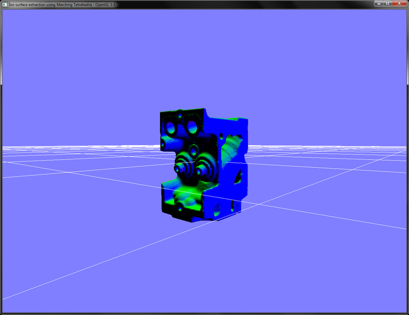
Pressing the W key toggles the wireframe display, which shows the underlying isosurface polygons for isovalue of 40 as shown in the following screenshot:

While in this recipe, we focused on the Marching Tetrahedra algorithm. There is another, more robust method of triangulation called Marching Cubes, which gives a more robust polygonisation as compared to the Marching Tetrahedra algorithm.
- Polygonising a scalar field, Paul Bourke: http://paulbourke.net/geometry/polygonise/
- Volume Rendering: Marching Cubes Algorithm, http://cns-alumni.bu.edu/~lavanya/Graphics/cs580/p5/web-page/p5.html
- An implementation of Marching Cubes and Marching Tetrahedra Algorithms, http://www.siafoo.net/snippet/100
Chapter7/MarchingTetrahedra directory. For convenience, we will wrap the Marching Tetrahedra algorithm in a simple class called TetrahedraMarcher.
Let us start this recipe by following these simple steps:
- Load the 3D volume data and store it into an array:
std::ifstream infile(filename.c_str(), std::ios_base::binary); if(infile.good()) { pVolume = new GLubyte[XDIM*YDIM*ZDIM]; infile.read(reinterpret_cast<char*>(pVolume), XDIM*YDIM*ZDIM*sizeof(GLubyte)); infile.close(); return true; } else { return false; } - Depending on the sampling box size, run three loops to iterate through the entire volume voxel by voxel:
vertices.clear(); int dx = XDIM/X_SAMPLING_DIST; int dy = YDIM/Y_SAMPLING_DIST; int dz = ZDIM/Z_SAMPLING_DIST; glm::vec3 scale = glm::vec3(dx,dy,dz); for(int z=0;z<ZDIM;z+=dz) { for(int y=0;y<YDIM;y+=dy) { for(int x=0;x<XDIM;x+=dx) { SampleVoxel(x,y,z, scale); } } } - In each sampling step, estimate the volume density values at the eight corners of the sampling box:
GLubyte cubeCornerValues[8]; for( i = 0; i < 8; i++) { cubeCornerValues[i] = SampleVolume( x + (int)(a2fVertexOffset[i][0] *scale.x), y + (int)(a2fVertexOffset[i][1]*scale.y), z + (int)(a2fVertexOffset[i][2]*scale.z)); } - Estimate an edge flag value to identify the matching tetrahedra case based on the given isovalue:
int flagIndex = 0; for( i= 0; i<8; i++) { if(cubeCornerValues[i]<= isoValue) flagIndex |= 1<<i; } edgeFlags = aiCubeEdgeFlags[flagIndex]; - Use the lookup tables (
a2iEdgeConnection) to find the correct edges for the case and then use the offset table (a2fVertexOffset) to find the edge vertices and normals. These tables are defined in theTables.hheader in theChapter7/MarchingTetrahedra/directory.for(i = 0; i < 12; i++) { if(edgeFlags & (1<<i)) { float offset = GetOffset(cubeCornerValues[ a2iEdgeConnection[i][0] ], cubeCornerValues[ a2iEdgeConnection[i][1] ]); edgeVertices[i].x = x + (a2fVertexOffset[ a2iEdgeConnection[i][0] ][0] + offset * a2fEdgeDirection[i][0])*scale.x ; edgeVertices[i].y = y + (a2fVertexOffset[ a2iEdgeConnection[i][0] ][1] + offset * a2fEdgeDirection[i][1])*scale.y ; edgeVertices[i].z = z + (a2fVertexOffset[ a2iEdgeConnection[i][0] ][2] + offset * a2fEdgeDirection[i][2])*scale.z ; edgeNormals[i] = GetNormal( (int)edgeVertices[i].x , (int)edgeVertices[i].y , (int)edgeVertices[i].z ); } } - Finally, loop through the triangle connectivity table to connect the correct vertices and normals for the given case.
for(i = 0; i< 5; i++) { if(a2iTriangleConnectionTable[flagIndex][3*i] < 0) break; for(int j= 0; j< 3; j++) { int vertex = a2iTriangleConnectionTable[flagIndex][3*i+j]; Vertex v; v.normal = (edgeNormals[vertex]); v.pos = (edgeVertices[vertex])*invDim; vertices.push_back(v); } } - After the marcher is finished, we pass the generated vertices to a vertex array object containing a vertex buffer object:
glGenVertexArrays(1, &volumeMarcherVAO); glGenBuffers(1, &volumeMarcherVBO); glBindVertexArray(volumeMarcherVAO); glBindBuffer (GL_ARRAY_BUFFER, volumeMarcherVBO); glBufferData (GL_ARRAY_BUFFER, marcher-> GetTotalVertices()*sizeof(Vertex), marcher-> GetVertexPointer(), GL_STATIC_DRAW); glEnableVertexAttribArray(0); glVertexAttribPointer(0, 3, GL_FLOAT, GL_FALSE,sizeof(Vertex),0); glEnableVertexAttribArray(1); glVertexAttribPointer(1, 3, GL_FLOAT, GL_FALSE,sizeof(Vertex),(const GLvoid*)offsetof(Vertex, normal));
- For rendering of the generated geometry, we bind the Marching Tetrahedra VAO, bind our shader and then render the triangles. For this recipe, we output the per-vertex normals as color.
glBindVertexArray(volumeMarcherVAO); shader.Use(); glUniformMatrix4fv(shader("MVP"),1,GL_FALSE, glm::value_ptr(MVP*T)); glDrawArrays(GL_TRIANGLES, 0, marcher->GetTotalVertices()); shader.UnUse();
For convenience, we wrap the entire recipe in a reusable class called TetrahedraMarcher. Marching Tetrahedra, as the name suggests, marches a sampling box throughout the whole volume dataset. To give a bird's eye view there are several cases to consider based on the distribution of density values at the vertices of the sampling cube. Based on the sampling values at the eight corners and the given isovalue, a flag index is generated. This flag index gives us the edge flag by a lookup in a table. This edge flag is then used in an edge lookup table, which is predefined for all possible edge configurations of the marching tetrahedron. The edge connection table is then used to find the appropriate offset for the corner values of the sampling box. These offsets are then used to obtain the edge vertices and normals for the given tetrahedral case. Once the list of edge vertices and normals are estimated, the triangle connectivity is obtained based on the given flag index.
Now we will detail the steps in the Marching Tetrahedra algorithm. First, the flag index is obtained by iterating through all eight sampling cube vertices and comparing the density value at the vertex location with the given isovalue as shown in the following code. The flag index is then used to retrieve the edge flags from the looktup table (aiCubeEdgeFlags).
After the Marching Tetrahedra code is processed, we store the generated vertices and normals in a buffer object. In the rendering code, we bind the appropriate vertex array object, bind our shader and then draw the triangles. The fragment shader for this recipe outputs the per-vertex normals as colors.
Pressing the W key toggles the wireframe display, which shows the underlying isosurface polygons for isovalue of 40 as shown in the following screenshot:
While in this recipe, we focused on the Marching Tetrahedra algorithm. There is another, more robust method of triangulation called Marching Cubes, which gives a more robust polygonisation as compared to the Marching Tetrahedra algorithm.
- Polygonising a scalar field, Paul Bourke: http://paulbourke.net/geometry/polygonise/
- Volume Rendering: Marching Cubes Algorithm, http://cns-alumni.bu.edu/~lavanya/Graphics/cs580/p5/web-page/p5.html
- An implementation of Marching Cubes and Marching Tetrahedra Algorithms, http://www.siafoo.net/snippet/100
recipe by following these simple steps:
- Load the 3D volume data and store it into an array:
std::ifstream infile(filename.c_str(), std::ios_base::binary); if(infile.good()) { pVolume = new GLubyte[XDIM*YDIM*ZDIM]; infile.read(reinterpret_cast<char*>(pVolume), XDIM*YDIM*ZDIM*sizeof(GLubyte)); infile.close(); return true; } else { return false; } - Depending on the sampling box size, run three loops to iterate through the entire volume voxel by voxel:
vertices.clear(); int dx = XDIM/X_SAMPLING_DIST; int dy = YDIM/Y_SAMPLING_DIST; int dz = ZDIM/Z_SAMPLING_DIST; glm::vec3 scale = glm::vec3(dx,dy,dz); for(int z=0;z<ZDIM;z+=dz) { for(int y=0;y<YDIM;y+=dy) { for(int x=0;x<XDIM;x+=dx) { SampleVoxel(x,y,z, scale); } } } - In each sampling step, estimate the volume density values at the eight corners of the sampling box:
GLubyte cubeCornerValues[8]; for( i = 0; i < 8; i++) { cubeCornerValues[i] = SampleVolume( x + (int)(a2fVertexOffset[i][0] *scale.x), y + (int)(a2fVertexOffset[i][1]*scale.y), z + (int)(a2fVertexOffset[i][2]*scale.z)); } - Estimate an edge flag value to identify the matching tetrahedra case based on the given isovalue:
int flagIndex = 0; for( i= 0; i<8; i++) { if(cubeCornerValues[i]<= isoValue) flagIndex |= 1<<i; } edgeFlags = aiCubeEdgeFlags[flagIndex]; - Use the lookup tables (
a2iEdgeConnection) to find the correct edges for the case and then use the offset table (a2fVertexOffset) to find the edge vertices and normals. These tables are defined in theTables.hheader in theChapter7/MarchingTetrahedra/directory.for(i = 0; i < 12; i++) { if(edgeFlags & (1<<i)) { float offset = GetOffset(cubeCornerValues[ a2iEdgeConnection[i][0] ], cubeCornerValues[ a2iEdgeConnection[i][1] ]); edgeVertices[i].x = x + (a2fVertexOffset[ a2iEdgeConnection[i][0] ][0] + offset * a2fEdgeDirection[i][0])*scale.x ; edgeVertices[i].y = y + (a2fVertexOffset[ a2iEdgeConnection[i][0] ][1] + offset * a2fEdgeDirection[i][1])*scale.y ; edgeVertices[i].z = z + (a2fVertexOffset[ a2iEdgeConnection[i][0] ][2] + offset * a2fEdgeDirection[i][2])*scale.z ; edgeNormals[i] = GetNormal( (int)edgeVertices[i].x , (int)edgeVertices[i].y , (int)edgeVertices[i].z ); } } - Finally, loop through the triangle connectivity table to connect the correct vertices and normals for the given case.
for(i = 0; i< 5; i++) { if(a2iTriangleConnectionTable[flagIndex][3*i] < 0) break; for(int j= 0; j< 3; j++) { int vertex = a2iTriangleConnectionTable[flagIndex][3*i+j]; Vertex v; v.normal = (edgeNormals[vertex]); v.pos = (edgeVertices[vertex])*invDim; vertices.push_back(v); } } - After the marcher is finished, we pass the generated vertices to a vertex array object containing a vertex buffer object:
glGenVertexArrays(1, &volumeMarcherVAO); glGenBuffers(1, &volumeMarcherVBO); glBindVertexArray(volumeMarcherVAO); glBindBuffer (GL_ARRAY_BUFFER, volumeMarcherVBO); glBufferData (GL_ARRAY_BUFFER, marcher-> GetTotalVertices()*sizeof(Vertex), marcher-> GetVertexPointer(), GL_STATIC_DRAW); glEnableVertexAttribArray(0); glVertexAttribPointer(0, 3, GL_FLOAT, GL_FALSE,sizeof(Vertex),0); glEnableVertexAttribArray(1); glVertexAttribPointer(1, 3, GL_FLOAT, GL_FALSE,sizeof(Vertex),(const GLvoid*)offsetof(Vertex, normal));
- For rendering of the generated geometry, we bind the Marching Tetrahedra VAO, bind our shader and then render the triangles. For this recipe, we output the per-vertex normals as color.
glBindVertexArray(volumeMarcherVAO); shader.Use(); glUniformMatrix4fv(shader("MVP"),1,GL_FALSE, glm::value_ptr(MVP*T)); glDrawArrays(GL_TRIANGLES, 0, marcher->GetTotalVertices()); shader.UnUse();
For convenience, we wrap the entire recipe in a reusable class called TetrahedraMarcher. Marching Tetrahedra, as the name suggests, marches a sampling box throughout the whole volume dataset. To give a bird's eye view there are several cases to consider based on the distribution of density values at the vertices of the sampling cube. Based on the sampling values at the eight corners and the given isovalue, a flag index is generated. This flag index gives us the edge flag by a lookup in a table. This edge flag is then used in an edge lookup table, which is predefined for all possible edge configurations of the marching tetrahedron. The edge connection table is then used to find the appropriate offset for the corner values of the sampling box. These offsets are then used to obtain the edge vertices and normals for the given tetrahedral case. Once the list of edge vertices and normals are estimated, the triangle connectivity is obtained based on the given flag index.
Now we will detail the steps in the Marching Tetrahedra algorithm. First, the flag index is obtained by iterating through all eight sampling cube vertices and comparing the density value at the vertex location with the given isovalue as shown in the following code. The flag index is then used to retrieve the edge flags from the looktup table (aiCubeEdgeFlags).
After the Marching Tetrahedra code is processed, we store the generated vertices and normals in a buffer object. In the rendering code, we bind the appropriate vertex array object, bind our shader and then draw the triangles. The fragment shader for this recipe outputs the per-vertex normals as colors.
Pressing the W key toggles the wireframe display, which shows the underlying isosurface polygons for isovalue of 40 as shown in the following screenshot:
While in this recipe, we focused on the Marching Tetrahedra algorithm. There is another, more robust method of triangulation called Marching Cubes, which gives a more robust polygonisation as compared to the Marching Tetrahedra algorithm.
- Polygonising a scalar field, Paul Bourke: http://paulbourke.net/geometry/polygonise/
- Volume Rendering: Marching Cubes Algorithm, http://cns-alumni.bu.edu/~lavanya/Graphics/cs580/p5/web-page/p5.html
- An implementation of Marching Cubes and Marching Tetrahedra Algorithms, http://www.siafoo.net/snippet/100
TetrahedraMarcher. Marching Tetrahedra, as the name suggests, marches a sampling box throughout the whole volume dataset. To give a bird's eye view there are several cases to consider based on the distribution of density values at the vertices of the sampling cube. Based on the sampling values at the eight corners and the given isovalue, a flag index is generated. This flag index gives us the edge flag by a lookup in a table. This edge flag is then used in an edge lookup table, which is predefined for all possible edge configurations of the marching tetrahedron. The edge connection table is then used to find the appropriate offset for the corner values of the sampling box. These offsets are then used to obtain the edge vertices and normals for the given tetrahedral case. Once the list of edge vertices and
normals are estimated, the triangle connectivity is obtained based on the given flag index.
Now we will detail the steps in the Marching Tetrahedra algorithm. First, the flag index is obtained by iterating through all eight sampling cube vertices and comparing the density value at the vertex location with the given isovalue as shown in the following code. The flag index is then used to retrieve the edge flags from the looktup table (aiCubeEdgeFlags).
After the Marching Tetrahedra code is processed, we store the generated vertices and normals in a buffer object. In the rendering code, we bind the appropriate vertex array object, bind our shader and then draw the triangles. The fragment shader for this recipe outputs the per-vertex normals as colors.
Pressing the W key toggles the wireframe display, which shows the underlying isosurface polygons for isovalue of 40 as shown in the following screenshot:
While in this recipe, we focused on the Marching Tetrahedra algorithm. There is another, more robust method of triangulation called Marching Cubes, which gives a more robust polygonisation as compared to the Marching Tetrahedra algorithm.
- Polygonising a scalar field, Paul Bourke: http://paulbourke.net/geometry/polygonise/
- Volume Rendering: Marching Cubes Algorithm, http://cns-alumni.bu.edu/~lavanya/Graphics/cs580/p5/web-page/p5.html
- An implementation of Marching Cubes and Marching Tetrahedra Algorithms, http://www.siafoo.net/snippet/100
toggles the wireframe display, which shows the underlying isosurface polygons for isovalue of 40 as shown in the following screenshot:
While in this recipe, we focused on the Marching Tetrahedra algorithm. There is another, more robust method of triangulation called Marching Cubes, which gives a more robust polygonisation as compared to the Marching Tetrahedra algorithm.
- Polygonising a scalar field, Paul Bourke: http://paulbourke.net/geometry/polygonise/
- Volume Rendering: Marching Cubes Algorithm, http://cns-alumni.bu.edu/~lavanya/Graphics/cs580/p5/web-page/p5.html
- An implementation of Marching Cubes and Marching Tetrahedra Algorithms, http://www.siafoo.net/snippet/100
- http://paulbourke.net/geometry/polygonise/
- Volume Rendering: Marching Cubes Algorithm, http://cns-alumni.bu.edu/~lavanya/Graphics/cs580/p5/web-page/p5.html
- An implementation of Marching Cubes and Marching Tetrahedra Algorithms, http://www.siafoo.net/snippet/100
In this recipe, we will implement volumetric lighting using the half-angle slicing technique. Instead of slicing the volume perpendicular to the viewing direction, the slicing direction is set between the light and the view direction vectors. This enables us to simulate light absorption slice by slice.
Let us start this recipe by following these simple steps:
- Setup offscreen rendering using one FBO with two attachments: one for offscreen rendering of the light buffer and the other for offscreen rendering of the eye buffer.
glGenFramebuffers(1, &lightFBOID); glGenTextures (1, &lightBufferID); glGenTextures (1, &eyeBufferID); glActiveTexture(GL_TEXTURE2); lightBufferID = CreateTexture(IMAGE_WIDTH, IMAGE_HEIGHT, GL_RGBA16F, GL_RGBA); eyeBufferID = CreateTexture(IMAGE_WIDTH, IMAGE_HEIGHT, GL_RGBA16F, GL_RGBA); glBindFramebuffer(GL_FRAMEBUFFER, lightFBOID); glFramebufferTexture2D(GL_FRAMEBUFFER, GL_COLOR_ATTACHMENT0, GL_TEXTURE_2D, lightBufferID, 0); glFramebufferTexture2D(GL_FRAMEBUFFER, GL_COLOR_ATTACHMENT1, GL_TEXTURE_2D, eyeBufferID, 0); GLenum status = glCheckFramebufferStatus(GL_FRAMEBUFFER); if(status == GL_FRAMEBUFFER_COMPLETE ) printf("Light FBO setup successful !!! \n"); else printf("Problem with Light FBO setup");
The
CreateTexturefunction performs the texture creation and texture format specification into a single function for convenience. This function is defined as follows: - Load the volume data, as in the 3D texture slicing recipe:
std::ifstream infile(volume_file.c_str(), std::ios_base::binary); if(infile.good()) { GLubyte* pData = new GLubyte[XDIM*YDIM*ZDIM]; infile.read(reinterpret_cast<char*>(pData), XDIM*YDIM*ZDIM*sizeof(GLubyte)); infile.close(); glGenTextures(1, &textureID); glActiveTexture(GL_TEXTURE0); glBindTexture(GL_TEXTURE_3D, textureID); // set the texture parameters glTexImage3D(GL_TEXTURE_3D,0,GL_RED,XDIM,YDIM,ZDIM,0, GL_RED,GL_UNSIGNED_BYTE,pData); GL_CHECK_ERRORS glGenerateMipmap(GL_TEXTURE_3D); return true; } else { return false; } - Similar to the shadow mapping technique, calculate the shadow matrix by multiplying the model-view and projection matrices of the light with the bias matrix:
MV_L=glm::lookAt(lightPosOS,glm::vec3(0,0,0), glm::vec3(0,1,0)); P_L=glm::perspective(45.0f,1.0f,1.0f, 200.0f); B=glm::scale(glm::translate(glm::mat4(1), glm::vec3(0.5,0.5,0.5)), glm::vec3(0.5,0.5,0.5)); BP = B*P_L; S = BP*MV_L; - In the rendering code, calculate the half vector by using the view direction vector and the light direction vector:
viewVec = -glm::vec3(MV[0][2], MV[1][2], MV[2][2]); lightVec = glm::normalize(lightPosOS); bIsViewInverted = glm::dot(viewVec, lightVec)<0; halfVec = glm::normalize( (bIsViewInverted?-viewVec:viewVec) + lightVec);
- Slice the volume data as in the 3D texture slicing recipe. The only difference here is that instead of slicing the volume data in the direction perpendicular to the view, we slice it in the direction which is halfway between the view and the light vectors.
float max_dist = glm::dot(halfVec, vertexList[0]); float min_dist = max_dist; int max_index = 0; int count = 0; for(int i=1;i<8;i++) { float dist = glm::dot(halfVec, vertexList[i]); if(dist > max_dist) { max_dist = dist; max_index = i; } if(dist<min_dist) min_dist = dist; } //rest of the SliceVolume function as in 3D texture slicing but //viewVec is changed to halfVec
- In the rendering code, bind the FBO and then first clear the light buffer with the white
color (1,1,1,1)and the eye buffer with thecolor (0,0,0,0):glBindFramebuffer(GL_FRAMEBUFFER, lightFBOID); glDrawBuffer(attachIDs[0]); glClearColor(1,1,1,1); glClear(GL_COLOR_BUFFER_BIT ); glDrawBuffer(attachIDs[1]); glClearColor(0,0,0,0); glClear(GL_COLOR_BUFFER_BIT );
- Bind the volume VAO and then run a loop for the total number of slices. In each iteration, first render the slice in the eye buffer but bind the light buffer as the texture. Next, render the slice in the light buffer:
glBindVertexArray(volumeVAO); for(int i =0;i<num_slices;i++) { shaderShadow.Use(); glUniformMatrix4fv(shaderShadow("MVP"), 1, GL_FALSE, glm::value_ptr(MVP)); glUniformMatrix4fv(shaderShadow("S"), 1, GL_FALSE, glm::value_ptr(S)); glBindTexture(GL_TEXTURE_2D, lightBuffer); DrawSliceFromEyePointOfView(i); shader.Use(); glUniformMatrix4fv(shader("MVP"), 1, GL_FALSE, glm::value_ptr(P_L*MV_L)); DrawSliceFromLightPointOfView(i); } - For the eye buffer rendering step, swap the blend function based on whether the viewer is viewing in the direction of the light or opposite to it:
void DrawSliceFromEyePointOfView(const int i) { glDrawBuffer(attachIDs[1]); glViewport(0, 0, IMAGE_WIDTH, IMAGE_HEIGHT); if(bIsViewInverted) { glBlendFunc(GL_ONE_MINUS_DST_ALPHA, GL_ONE); } else { glBlendFunc(GL_ONE, GL_ONE_MINUS_SRC_ALPHA); } glDrawArrays(GL_TRIANGLES, 12*i, 12); } - For the light buffer, we simply blend the slices using the conventional "over" blending:
void DrawSliceFromLightPointOfView(const int i) { glDrawBuffer(attachIDs[0]); glViewport(0, 0, IMAGE_WIDTH, IMAGE_HEIGHT); glBlendFunc(GL_SRC_ALPHA, GL_ONE_MINUS_SRC_ALPHA); glDrawArrays(GL_TRIANGLES, 12*i, 12); } - Finally, unbind the FBO and restore the default draw buffer. Next, set the viewport to the entire screen and then render the eye buffer on screen using a shader:
glBindVertexArray(0); glBindFramebuffer(GL_FRAMEBUFFER, 0); glDrawBuffer(GL_BACK_LEFT); glViewport(0,0,WIDTH, HEIGHT); glBindTexture(GL_TEXTURE_2D, eyeBufferID); glBindVertexArray(quadVAOID); quadShader.Use(); glDrawArrays(GL_TRIANGLES, 0, 6); quadShader.UnUse(); glBindVertexArray(0);
As the name suggests, this technique renders the volume by accumulating the intermediate results into two separate buffers by slicing the volume halfway between the light and the view vectors. When the scene is rendered from the point of view of the eye, the light buffer is used as texture to find out whether the current fragment is in shadow or not. This is carried out in the fragment shader by looking up the light buffer by using the shadow matrix as in the shadow mapping algorithm. In this step, the blending equation is swapped based on the direction of view with respect to the light direction vector. If the view is inverted, the blending direction is swapped from front-to-back to back-to-front using glBlendFunc(GL_ONE_MINUS_DST_ALPHA, GL_ONE). On the other hand, if the view direction is not inverted, the blend function is set as glBlendFunc(GL_ONE, GL_ONE_MINUS_SRC_ALPHA). Note that here we have not used the over compositing since we premultiply the color with its alpha in the fragment shader (see Chapter7/HalfAngleSlicing/shaders/slicerShadow.frag), as shown in the following code:
In the next step, the scene is rendered from the point of view of the light. This time, the normal over compositing is used. This ensures that the light contributions accumulate with each other similar to how light behaves in normal circumstances. In this case, we use the same fragment shader as was used in the 3D texture slicing recipe (see Chapter7/HalgAngleSlicing/shaders/textureSlicer.frag).
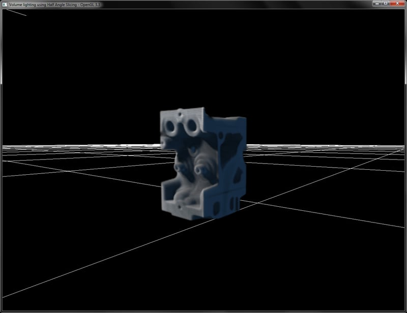
Note that we cannot see the black halo around the volume dataset as was evident in earlier recipes. The reason for this is the if condition used in the fragment shader. We only perform these calculations if the current density value is greater than 0.1. This essentially removed air and other low intensity artifacts, producing a much better result.
- Chapter 39, Volume Rendering Techniques, in GPU Gems 1. Available online at http://http.developer.nvidia.com/GPUGems/gpugems_ch39.html
- Chapter 6, Global Volume Illumination, in Real-time Volume Graphics, AK Peters/CRC Press.
Chapter7/HalfAngleSlicing directory. As the name suggests, this recipe will build up on the 3D texture slicing code.
Let us start this recipe by following these simple steps:
- Setup offscreen rendering using one FBO with two attachments: one for offscreen rendering of the light buffer and the other for offscreen rendering of the eye buffer.
glGenFramebuffers(1, &lightFBOID); glGenTextures (1, &lightBufferID); glGenTextures (1, &eyeBufferID); glActiveTexture(GL_TEXTURE2); lightBufferID = CreateTexture(IMAGE_WIDTH, IMAGE_HEIGHT, GL_RGBA16F, GL_RGBA); eyeBufferID = CreateTexture(IMAGE_WIDTH, IMAGE_HEIGHT, GL_RGBA16F, GL_RGBA); glBindFramebuffer(GL_FRAMEBUFFER, lightFBOID); glFramebufferTexture2D(GL_FRAMEBUFFER, GL_COLOR_ATTACHMENT0, GL_TEXTURE_2D, lightBufferID, 0); glFramebufferTexture2D(GL_FRAMEBUFFER, GL_COLOR_ATTACHMENT1, GL_TEXTURE_2D, eyeBufferID, 0); GLenum status = glCheckFramebufferStatus(GL_FRAMEBUFFER); if(status == GL_FRAMEBUFFER_COMPLETE ) printf("Light FBO setup successful !!! \n"); else printf("Problem with Light FBO setup");
The
CreateTexturefunction performs the texture creation and texture format specification into a single function for convenience. This function is defined as follows: - Load the volume data, as in the 3D texture slicing recipe:
std::ifstream infile(volume_file.c_str(), std::ios_base::binary); if(infile.good()) { GLubyte* pData = new GLubyte[XDIM*YDIM*ZDIM]; infile.read(reinterpret_cast<char*>(pData), XDIM*YDIM*ZDIM*sizeof(GLubyte)); infile.close(); glGenTextures(1, &textureID); glActiveTexture(GL_TEXTURE0); glBindTexture(GL_TEXTURE_3D, textureID); // set the texture parameters glTexImage3D(GL_TEXTURE_3D,0,GL_RED,XDIM,YDIM,ZDIM,0, GL_RED,GL_UNSIGNED_BYTE,pData); GL_CHECK_ERRORS glGenerateMipmap(GL_TEXTURE_3D); return true; } else { return false; } - Similar to the shadow mapping technique, calculate the shadow matrix by multiplying the model-view and projection matrices of the light with the bias matrix:
MV_L=glm::lookAt(lightPosOS,glm::vec3(0,0,0), glm::vec3(0,1,0)); P_L=glm::perspective(45.0f,1.0f,1.0f, 200.0f); B=glm::scale(glm::translate(glm::mat4(1), glm::vec3(0.5,0.5,0.5)), glm::vec3(0.5,0.5,0.5)); BP = B*P_L; S = BP*MV_L; - In the rendering code, calculate the half vector by using the view direction vector and the light direction vector:
viewVec = -glm::vec3(MV[0][2], MV[1][2], MV[2][2]); lightVec = glm::normalize(lightPosOS); bIsViewInverted = glm::dot(viewVec, lightVec)<0; halfVec = glm::normalize( (bIsViewInverted?-viewVec:viewVec) + lightVec);
- Slice the volume data as in the 3D texture slicing recipe. The only difference here is that instead of slicing the volume data in the direction perpendicular to the view, we slice it in the direction which is halfway between the view and the light vectors.
float max_dist = glm::dot(halfVec, vertexList[0]); float min_dist = max_dist; int max_index = 0; int count = 0; for(int i=1;i<8;i++) { float dist = glm::dot(halfVec, vertexList[i]); if(dist > max_dist) { max_dist = dist; max_index = i; } if(dist<min_dist) min_dist = dist; } //rest of the SliceVolume function as in 3D texture slicing but //viewVec is changed to halfVec
- In the rendering code, bind the FBO and then first clear the light buffer with the white
color (1,1,1,1)and the eye buffer with thecolor (0,0,0,0):glBindFramebuffer(GL_FRAMEBUFFER, lightFBOID); glDrawBuffer(attachIDs[0]); glClearColor(1,1,1,1); glClear(GL_COLOR_BUFFER_BIT ); glDrawBuffer(attachIDs[1]); glClearColor(0,0,0,0); glClear(GL_COLOR_BUFFER_BIT );
- Bind the volume VAO and then run a loop for the total number of slices. In each iteration, first render the slice in the eye buffer but bind the light buffer as the texture. Next, render the slice in the light buffer:
glBindVertexArray(volumeVAO); for(int i =0;i<num_slices;i++) { shaderShadow.Use(); glUniformMatrix4fv(shaderShadow("MVP"), 1, GL_FALSE, glm::value_ptr(MVP)); glUniformMatrix4fv(shaderShadow("S"), 1, GL_FALSE, glm::value_ptr(S)); glBindTexture(GL_TEXTURE_2D, lightBuffer); DrawSliceFromEyePointOfView(i); shader.Use(); glUniformMatrix4fv(shader("MVP"), 1, GL_FALSE, glm::value_ptr(P_L*MV_L)); DrawSliceFromLightPointOfView(i); } - For the eye buffer rendering step, swap the blend function based on whether the viewer is viewing in the direction of the light or opposite to it:
void DrawSliceFromEyePointOfView(const int i) { glDrawBuffer(attachIDs[1]); glViewport(0, 0, IMAGE_WIDTH, IMAGE_HEIGHT); if(bIsViewInverted) { glBlendFunc(GL_ONE_MINUS_DST_ALPHA, GL_ONE); } else { glBlendFunc(GL_ONE, GL_ONE_MINUS_SRC_ALPHA); } glDrawArrays(GL_TRIANGLES, 12*i, 12); } - For the light buffer, we simply blend the slices using the conventional "over" blending:
void DrawSliceFromLightPointOfView(const int i) { glDrawBuffer(attachIDs[0]); glViewport(0, 0, IMAGE_WIDTH, IMAGE_HEIGHT); glBlendFunc(GL_SRC_ALPHA, GL_ONE_MINUS_SRC_ALPHA); glDrawArrays(GL_TRIANGLES, 12*i, 12); } - Finally, unbind the FBO and restore the default draw buffer. Next, set the viewport to the entire screen and then render the eye buffer on screen using a shader:
glBindVertexArray(0); glBindFramebuffer(GL_FRAMEBUFFER, 0); glDrawBuffer(GL_BACK_LEFT); glViewport(0,0,WIDTH, HEIGHT); glBindTexture(GL_TEXTURE_2D, eyeBufferID); glBindVertexArray(quadVAOID); quadShader.Use(); glDrawArrays(GL_TRIANGLES, 0, 6); quadShader.UnUse(); glBindVertexArray(0);
As the name suggests, this technique renders the volume by accumulating the intermediate results into two separate buffers by slicing the volume halfway between the light and the view vectors. When the scene is rendered from the point of view of the eye, the light buffer is used as texture to find out whether the current fragment is in shadow or not. This is carried out in the fragment shader by looking up the light buffer by using the shadow matrix as in the shadow mapping algorithm. In this step, the blending equation is swapped based on the direction of view with respect to the light direction vector. If the view is inverted, the blending direction is swapped from front-to-back to back-to-front using glBlendFunc(GL_ONE_MINUS_DST_ALPHA, GL_ONE). On the other hand, if the view direction is not inverted, the blend function is set as glBlendFunc(GL_ONE, GL_ONE_MINUS_SRC_ALPHA). Note that here we have not used the over compositing since we premultiply the color with its alpha in the fragment shader (see Chapter7/HalfAngleSlicing/shaders/slicerShadow.frag), as shown in the following code:
In the next step, the scene is rendered from the point of view of the light. This time, the normal over compositing is used. This ensures that the light contributions accumulate with each other similar to how light behaves in normal circumstances. In this case, we use the same fragment shader as was used in the 3D texture slicing recipe (see Chapter7/HalgAngleSlicing/shaders/textureSlicer.frag).
Note that we cannot see the black halo around the volume dataset as was evident in earlier recipes. The reason for this is the if condition used in the fragment shader. We only perform these calculations if the current density value is greater than 0.1. This essentially removed air and other low intensity artifacts, producing a much better result.
- Chapter 39, Volume Rendering Techniques, in GPU Gems 1. Available online at http://http.developer.nvidia.com/GPUGems/gpugems_ch39.html
- Chapter 6, Global Volume Illumination, in Real-time Volume Graphics, AK Peters/CRC Press.
glGenFramebuffers(1, &lightFBOID); glGenTextures (1, &lightBufferID); glGenTextures (1, &eyeBufferID); glActiveTexture(GL_TEXTURE2); lightBufferID = CreateTexture(IMAGE_WIDTH, IMAGE_HEIGHT, GL_RGBA16F, GL_RGBA); eyeBufferID = CreateTexture(IMAGE_WIDTH, IMAGE_HEIGHT, GL_RGBA16F, GL_RGBA); glBindFramebuffer(GL_FRAMEBUFFER, lightFBOID); glFramebufferTexture2D(GL_FRAMEBUFFER, GL_COLOR_ATTACHMENT0, GL_TEXTURE_2D, lightBufferID, 0); glFramebufferTexture2D(GL_FRAMEBUFFER, GL_COLOR_ATTACHMENT1, GL_TEXTURE_2D, eyeBufferID, 0); GLenum status = glCheckFramebufferStatus(GL_FRAMEBUFFER); if(status == GL_FRAMEBUFFER_COMPLETE ) printf("Light FBO setup successful !!! \n"); else printf("Problem with Light FBO setup");
CreateTexture function
performs the texture creation and texture format specification into a single function for convenience. This function is defined as follows:
- Load the volume data, as in the 3D texture slicing recipe:
std::ifstream infile(volume_file.c_str(), std::ios_base::binary); if(infile.good()) { GLubyte* pData = new GLubyte[XDIM*YDIM*ZDIM]; infile.read(reinterpret_cast<char*>(pData), XDIM*YDIM*ZDIM*sizeof(GLubyte)); infile.close(); glGenTextures(1, &textureID); glActiveTexture(GL_TEXTURE0); glBindTexture(GL_TEXTURE_3D, textureID); // set the texture parameters glTexImage3D(GL_TEXTURE_3D,0,GL_RED,XDIM,YDIM,ZDIM,0, GL_RED,GL_UNSIGNED_BYTE,pData); GL_CHECK_ERRORS glGenerateMipmap(GL_TEXTURE_3D); return true; } else { return false; } - Similar to the shadow mapping technique, calculate the shadow matrix by multiplying the model-view and projection matrices of the light with the bias matrix:
MV_L=glm::lookAt(lightPosOS,glm::vec3(0,0,0), glm::vec3(0,1,0)); P_L=glm::perspective(45.0f,1.0f,1.0f, 200.0f); B=glm::scale(glm::translate(glm::mat4(1), glm::vec3(0.5,0.5,0.5)), glm::vec3(0.5,0.5,0.5)); BP = B*P_L; S = BP*MV_L; - In the rendering code, calculate the half vector by using the view direction vector and the light direction vector:
viewVec = -glm::vec3(MV[0][2], MV[1][2], MV[2][2]); lightVec = glm::normalize(lightPosOS); bIsViewInverted = glm::dot(viewVec, lightVec)<0; halfVec = glm::normalize( (bIsViewInverted?-viewVec:viewVec) + lightVec);
- Slice the volume data as in the 3D texture slicing recipe. The only difference here is that instead of slicing the volume data in the direction perpendicular to the view, we slice it in the direction which is halfway between the view and the light vectors.
float max_dist = glm::dot(halfVec, vertexList[0]); float min_dist = max_dist; int max_index = 0; int count = 0; for(int i=1;i<8;i++) { float dist = glm::dot(halfVec, vertexList[i]); if(dist > max_dist) { max_dist = dist; max_index = i; } if(dist<min_dist) min_dist = dist; } //rest of the SliceVolume function as in 3D texture slicing but //viewVec is changed to halfVec
- In the rendering code, bind the FBO and then first clear the light buffer with the white
color (1,1,1,1)and the eye buffer with thecolor (0,0,0,0):glBindFramebuffer(GL_FRAMEBUFFER, lightFBOID); glDrawBuffer(attachIDs[0]); glClearColor(1,1,1,1); glClear(GL_COLOR_BUFFER_BIT ); glDrawBuffer(attachIDs[1]); glClearColor(0,0,0,0); glClear(GL_COLOR_BUFFER_BIT );
- Bind the volume VAO and then run a loop for the total number of slices. In each iteration, first render the slice in the eye buffer but bind the light buffer as the texture. Next, render the slice in the light buffer:
glBindVertexArray(volumeVAO); for(int i =0;i<num_slices;i++) { shaderShadow.Use(); glUniformMatrix4fv(shaderShadow("MVP"), 1, GL_FALSE, glm::value_ptr(MVP)); glUniformMatrix4fv(shaderShadow("S"), 1, GL_FALSE, glm::value_ptr(S)); glBindTexture(GL_TEXTURE_2D, lightBuffer); DrawSliceFromEyePointOfView(i); shader.Use(); glUniformMatrix4fv(shader("MVP"), 1, GL_FALSE, glm::value_ptr(P_L*MV_L)); DrawSliceFromLightPointOfView(i); } - For the eye buffer rendering step, swap the blend function based on whether the viewer is viewing in the direction of the light or opposite to it:
void DrawSliceFromEyePointOfView(const int i) { glDrawBuffer(attachIDs[1]); glViewport(0, 0, IMAGE_WIDTH, IMAGE_HEIGHT); if(bIsViewInverted) { glBlendFunc(GL_ONE_MINUS_DST_ALPHA, GL_ONE); } else { glBlendFunc(GL_ONE, GL_ONE_MINUS_SRC_ALPHA); } glDrawArrays(GL_TRIANGLES, 12*i, 12); } - For the light buffer, we simply blend the slices using the conventional "over" blending:
void DrawSliceFromLightPointOfView(const int i) { glDrawBuffer(attachIDs[0]); glViewport(0, 0, IMAGE_WIDTH, IMAGE_HEIGHT); glBlendFunc(GL_SRC_ALPHA, GL_ONE_MINUS_SRC_ALPHA); glDrawArrays(GL_TRIANGLES, 12*i, 12); } - Finally, unbind the FBO and restore the default draw buffer. Next, set the viewport to the entire screen and then render the eye buffer on screen using a shader:
glBindVertexArray(0); glBindFramebuffer(GL_FRAMEBUFFER, 0); glDrawBuffer(GL_BACK_LEFT); glViewport(0,0,WIDTH, HEIGHT); glBindTexture(GL_TEXTURE_2D, eyeBufferID); glBindVertexArray(quadVAOID); quadShader.Use(); glDrawArrays(GL_TRIANGLES, 0, 6); quadShader.UnUse(); glBindVertexArray(0);
As the name suggests, this technique renders the volume by accumulating the intermediate results into two separate buffers by slicing the volume halfway between the light and the view vectors. When the scene is rendered from the point of view of the eye, the light buffer is used as texture to find out whether the current fragment is in shadow or not. This is carried out in the fragment shader by looking up the light buffer by using the shadow matrix as in the shadow mapping algorithm. In this step, the blending equation is swapped based on the direction of view with respect to the light direction vector. If the view is inverted, the blending direction is swapped from front-to-back to back-to-front using glBlendFunc(GL_ONE_MINUS_DST_ALPHA, GL_ONE). On the other hand, if the view direction is not inverted, the blend function is set as glBlendFunc(GL_ONE, GL_ONE_MINUS_SRC_ALPHA). Note that here we have not used the over compositing since we premultiply the color with its alpha in the fragment shader (see Chapter7/HalfAngleSlicing/shaders/slicerShadow.frag), as shown in the following code:
In the next step, the scene is rendered from the point of view of the light. This time, the normal over compositing is used. This ensures that the light contributions accumulate with each other similar to how light behaves in normal circumstances. In this case, we use the same fragment shader as was used in the 3D texture slicing recipe (see Chapter7/HalgAngleSlicing/shaders/textureSlicer.frag).
Note that we cannot see the black halo around the volume dataset as was evident in earlier recipes. The reason for this is the if condition used in the fragment shader. We only perform these calculations if the current density value is greater than 0.1. This essentially removed air and other low intensity artifacts, producing a much better result.
- Chapter 39, Volume Rendering Techniques, in GPU Gems 1. Available online at http://http.developer.nvidia.com/GPUGems/gpugems_ch39.html
- Chapter 6, Global Volume Illumination, in Real-time Volume Graphics, AK Peters/CRC Press.
technique renders the volume by accumulating the intermediate results into two separate buffers by slicing the volume halfway between the light and the view vectors. When the scene is rendered from the point of view of the eye, the light buffer is used as texture to find out whether the current fragment is in shadow or not. This is carried out in the fragment shader by looking up the light buffer by using the shadow matrix as in the shadow mapping algorithm. In this step, the blending equation is swapped based on the direction of view with respect to the light direction vector. If the view is inverted, the blending direction is swapped from front-to-back to back-to-front using glBlendFunc(GL_ONE_MINUS_DST_ALPHA, GL_ONE). On the other hand, if the view direction is not inverted, the blend function is set as glBlendFunc(GL_ONE, GL_ONE_MINUS_SRC_ALPHA). Note that here we have not used the over compositing since we premultiply the color with its alpha in the fragment shader (see Chapter7/HalfAngleSlicing/shaders/slicerShadow.frag), as shown in the following code:
In the next step, the scene is rendered from the point of view of the light. This time, the normal over compositing is used. This ensures that the light contributions accumulate with each other similar to how light behaves in normal circumstances. In this case, we use the same fragment shader as was used in the 3D texture slicing recipe (see Chapter7/HalgAngleSlicing/shaders/textureSlicer.frag).
Note that we cannot see the black halo around the volume dataset as was evident in earlier recipes. The reason for this is the if condition used in the fragment shader. We only perform these calculations if the current density value is greater than 0.1. This essentially removed air and other low intensity artifacts, producing a much better result.
- Chapter 39, Volume Rendering Techniques, in GPU Gems 1. Available online at http://http.developer.nvidia.com/GPUGems/gpugems_ch39.html
- Chapter 6, Global Volume Illumination, in Real-time Volume Graphics, AK Peters/CRC Press.
- Chapter 39, Volume Rendering Techniques, in GPU Gems 1. Available online at http://http.developer.nvidia.com/GPUGems/gpugems_ch39.html
- Chapter 6, Global Volume Illumination, in Real-time Volume Graphics, AK Peters/CRC Press.
- http://http.developer.nvidia.com/GPUGems/gpugems_ch39.html
- Chapter 6, Global Volume Illumination, in Real-time Volume Graphics, AK Peters/CRC Press.