Before we can dive in and unlock the potential of GPUs, we first have to realize where their computational power lies in comparison to a modern Intel/AMD central processing unit (CPU)—the power does not lie in the fact that it has a higher clock speed than a CPU, nor in the complexity or particular design of the individual cores. An individual GPU core is actually quite simplistic, and at a disadvantage when compared to a modern individual CPU core, which use many fancy engineering tricks, such as branch prediction to reduce the latency of computations. Latency refers to the beginning-to-end duration of performing a single computation.

The power of the GPU derives from the fact that there are many, many more cores than in a CPU, which means a huge step forward in throughput. Throughput here refers to the number of computations that can be performed simultaneously. Let's use an analogy to get a better understanding of what this means. A GPU is like a very wide city road that is designed to handle many slower-moving cars at once (high throughput, high latency), whereas a CPU is like a narrow highway that can only admit a few cars at once, but can get each individual car to its destination much quicker (low throughput, low latency).

We can get an idea of the increase in throughput by seeing how many cores these new GPUs have. To give you an idea, the average Intel or AMD CPU has only two to eight cores—while an entry-level, consumer-grade NVIDIA GTX 1050 GPU has 640 cores, and a new top-of-the-line NVIDIA RTX 2080 Ti has 4,352 cores! We can exploit this massive throughput, provided we know how properly to parallelize any program or algorithm we wish to speed up. By parallelize, we mean to rewrite a program or algorithm so that we can split up our workload to run in parallel on multiple processors simultaneously. Let's think about an analogy from real-life.

Suppose that you are building a house and that you already have all of the designs and materials in place. You hire a single laborer, and you estimate it will take 100 hours to construct the house. Let's suppose that this particular house can be built in such a way that the work can be perfectly divided between every additional laborer you hire—that is to say, it will take 50 hours for two laborers, 25 hours for four laborers, and 10 hours for ten laborers to construct the house—the number of hours to construct your house will be 100 divided by the number of laborers you hire. This is an example of a parallelizable task.

We notice that this task is twice as fast to complete for two laborers, and ten times as fast for ten laborers to complete together (that is, in parallel) as opposed to one laborer building the house alone (that is, in serial)—that is, if N is the number of laborers, then it will be N times as fast. In this case, N is known as the speedup of parallelizing our task over the serial version of our task.

Before we begin to program a parallel version of a given algorithm, we often start by coming up with an estimate of the potential speedup that parallelization would bring to our task. This can help us determine whether it is worth expending resources and time writing a parallelization of our program or not. Because real life is more complicated than the example we gave here, it's pretty obvious that we won't be able to parallelize every program perfectly, all of the time—most of the time, only a part of our program will be nicely parallelizable, while the rest will have to run in serial.

We will now derive Amdahl's Law, which is a simple arithmetic formula that is used to estimate potential speed gain that may arise from parallelizing some portion of code from a serial program onto multiple processors. We will do this by continuing with our prior analogy of building a house.

Last time, we only considered the actual physical construction of the house as the entire time duration, but now, we will also consider the time it takes to design the house into the time duration for building the house. Suppose that only one person in the world has the ability to design your house—you—and it takes you 100 hours to design the plans for your house. There is no possibility that any other person on the planet can compare to your architectural brilliance, so there is no possibility that this part of the task can be split up at all between other architects—that is, so it will take 100 hours to design your house, regardless of what resources you have or how many people you can hire. So, if you have only one laborer to build your house, the entire time it will take to build your home will be 200 hours—100 hours for you to design it, and 100 hours for a single laborer to build it. If we hire two laborers, this will take 150 hours—the time to design the house will remain at 100 hours, while the construction will take 50 hours. It's clear that the total number of hours to construct the house will be 100 + 100 / N, where N is the number of laborers we hire.

Now, let's step back and think about how much time building the house takes if we hire one laborer—we ultimately use this to determine speedup as we hire additional laborers; that is, how many times faster the process becomes. If we hire a single laborer, we see that it takes the same amount of time to both design and construct the house—100 hours. So, we can say that that the portion of time spent on the design is .5 (50%), and the portion of the time it takes to construct the house is .5 (50%)—of course, both of these portions add up to 1, that is 100%. We want to make comparisons to this as we add laborers—if we have two laborers, the portion of time for the construction is halved, so in comparison to the original serial version of our task, this will take .5 + .5/2 = .75 (75%) of the time of the original task, and .75 x 200 hours is 150 hours, so we can see that this works. Moreover, we can see that if we have N laborers, we can calculate the percentage of time our parallelized construction with N laborers will take which the formula .5 + .5 / N.

Now, let's determine the speedup we are gaining by adding additional laborers. Since it takes 75% of the time to build a house if we have two laborers, we can take the reciprocal of .75 to determine the speedup of our parallelization—that is, the speedup will be 1 / .75, which is around 1.33 times faster than if we only have one laborer. In this case, we see that the speedup will be 1 / (.5 + .5 / N) if we have N laborers.

We know that .5 / N will shrink very close to 0 as we add more and more laborers, so we can see there is always an upper bound on the speedup you can get when you parallelize this task—that is, 1 / (.5 + 0) = 2. We can divide the original serial time with the estimated maximum speedup to determine an absolute minimum amount of time this task will take—200 / 2 = 100 hours.

The principle we have just applied to determine speedups in parallel programming is known as Amdahl's Law. It only requires knowledge of the parallelizable proportion of execution time for code in our original serial program, which is referred to as p, and the number of processor cores N that we have available.

We can now calculate speedup with Amdahl's Law as follows:

To sum it up, Amdahl's Law is a simple formula that allows us to roughly (very roughly) estimate potential speedup for a program that can be at least partially parallelized. This can provide a general idea as to whether it will be worthwhile to write a parallel version of a particular serial program, provided we know what proportion of the code we can parallelize (p), and how many cores we can run our parallelized code on (N).

We are now prepared to see a very standard example for parallel computing that we will revisit later in this text—an algorithm to generate an image of the Mandelbrot set. Let's first define exactly what we mean.

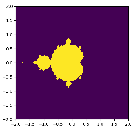
For a given complex number, c, we define a recursive sequence for , with and for . If |z_n| remains bounded by 2 as n increases to infinity, then we will say that c is a member of the Mandelbrot set.

Recall that we can visualize the complex numbers as residing on a two-dimensional Cartesian plane, with the x-axis representing the real components and the y-axis representing the imaginary components. We can therefore easily visualize the Mandelbrot set with a very appealing (and well-known) graph. Here, we will represent members of the Mandelbrot set with a lighter shade, and nonmembers with a darker shade on the complex Cartesian plane as follows:

Now, let's think about how we would go about generating this set in Python. We have to consider a few things first—since we obviously can't check whether every single complex number is in the Mandelbrot set, we have to choose a certain range to check over; we have to determine how many points in each range we will consider (width, height); and the maximum value of n that we will check |z_n| for (max_iters). We can now prepare to implement a function to generate a graph of the Mandelbrot set—here, we do this by iterating over every single point in the graph in serial.

We will start by importing the NumPy library, which is a numerical library that we will be making ample use of throughout this text. Our implementation here is in the simple_mandelbrot function. We start by using NumPy's linspace function to generate a lattice that will act as a discrete complex plane (the rest of the code that follows should be fairly straightforward):

import numpy as np

def simple_mandelbrot(width, height, real_low, real_high, imag_low, imag_high, max_iters):
    
     real_vals = np.linspace(real_low, real_high, width)
     imag_vals = np.linspace(imag_low, imag_high, height)
        
     # we will represent members as 1, non-members as 0.
    
     mandelbrot_graph = np.ones((height,width), dtype=np.float32)
    
     for x in range(width):
        
         for y in range(height):
            
             c = np.complex64( real_vals[x] + imag_vals[y] * 1j  )           
             z = np.complex64(0)
            
             for i in range(max_iters):
                
                 z = z**2 + c
                
                 if(np.abs(z) > 2):
                     mandelbrot_graph[y,x] = 0
                     break
                
     return mandelbrot_graph

Now, we want to add some code to dump the image of the Mandelbrot set to a PNG format file, so let's add the appropriate headers at the beginning:

from time import time
import matplotlib
# the following will prevent the figure from popping up
matplotlib.use('Agg')
from matplotlib import pyplot as plt

Now, let's add some code to generate the Mandelbrot set and dump it to a file, and use the time function to time both operations:

if __name__ == '__main__':
    
     t1 = time()
     mandel = simple_mandelbrot(512,512,-2,2,-2,2,256, 2)
     t2 = time()
     mandel_time = t2 - t1
    
     t1 = time()
     fig = plt.figure(1)
     plt.imshow(mandel, extent=(-2, 2, -2, 2))
     plt.savefig('mandelbrot.png', dpi=fig.dpi)
     t2 = time()
    
     dump_time = t2 - t1
    
     print 'It took {} seconds to calculate the Mandelbrot graph.'.format(mandel_time)
     print 'It took {} seconds to dump the image.'.format(dump_time)

Now let's run this program (this is also available as the mandelbrot0.py file, in folder 1, within the GitHub repository):

It took about 14.62 seconds to generate the Mandelbrot set, and about 0.11 seconds to dump the image. As we have seen, we generate the Mandelbrot set point by point; there is no interdependence between the values of different points, and it is, therefore, an intrinsically parallelizable function. In contrast, the code to dump the image cannot be parallelized.

Now, let's analyze this in terms of Amdahl's Law. What sort of speedups can we get if we parallelize our code here? In total, both pieces of the program took about 14.73 seconds to run; since we can parallelize the Mandelbrot set generation, we can say that the portion of execution time for parallelizable code is p = 14.62 / 14.73 = .99. This program is 99% parallelizable!

What sort of speedup can we potentially get? Well, I'm currently working on a laptop with an entry-level GTX 1050 GPU with 640 cores; our N will thus be 640 when we use the formula. We calculate the speedup as follows:

That is definitely very good and would indicate to us that it is worth our effort to program our algorithm to use the GPU. Keep in mind that Amdahl's Law only gives a very rough estimate! There will be additional considerations that will come into play when we offload computations onto the GPU, such as the additional time it takes for the CPU to send and receive data to and from the GPU; or the fact that algorithms that are offloaded to the GPU are only partially parallelizable.