Python Machine Learning Cookbook

Python Machine Learning Cookbook

By : Prateek Joshi, Vahid Mirjalili

Buy this Book

Python Machine Learning Cookbook

By: Prateek Joshi, Vahid Mirjalili

Buy this Book

Overview of this book

Machine learning is becoming increasingly pervasive in the modern data-driven world. It is used extensively across many fields such as search engines, robotics, self-driving cars, and more. With this book, you will learn how to perform various machine learning tasks in different environments. We’ll start by exploring a range of real-life scenarios where machine learning can be used, and look at various building blocks. Throughout the book, you’ll use a wide variety of machine learning algorithms to solve real-world problems and use Python to implement these algorithms. You’ll discover how to deal with various types of data and explore the differences between machine learning paradigms such as supervised and unsupervised learning. We also cover a range of regression techniques, classification algorithms, predictive modeling, data visualization techniques, recommendation engines, and more with the help of real-world examples.

Python Machine Learning Cookbook

Credits

About the Author

About the Reviewer

www.PacktPub.com

Preface

Free Chapter

The Realm of Supervised Learning

Introduction

Preprocessing data using different techniques

Label encoding

Building a linear regressor

Computing regression accuracy

Achieving model persistence

Building a ridge regressor

Building a polynomial regressor

Estimating housing prices

Computing the relative importance of features

Estimating bicycle demand distribution

Constructing a Classifier

Introduction

Building a simple classifier

Building a logistic regression classifier

Building a Naive Bayes classifier

Splitting the dataset for training and testing

Evaluating the accuracy using cross-validation

Visualizing the confusion matrix

Extracting the performance report

Evaluating cars based on their characteristics

Extracting validation curves

Extracting learning curves

Estimating the income bracket

Predictive Modeling

Introduction

Building a linear classifier using Support Vector Machine (SVMs)

Building a nonlinear classifier using SVMs

Tackling class imbalance

Extracting confidence measurements

Finding optimal hyperparameters

Building an event predictor

Estimating traffic

Clustering with Unsupervised Learning

Introduction

Clustering data using the k-means algorithm

Compressing an image using vector quantization

Building a Mean Shift clustering model

Grouping data using agglomerative clustering

Evaluating the performance of clustering algorithms

Automatically estimating the number of clusters using DBSCAN algorithm

Finding patterns in stock market data

Building a customer segmentation model

Building Recommendation Engines

Introduction

Building function compositions for data processing

Building machine learning pipelines

Finding the nearest neighbors

Constructing a k-nearest neighbors classifier

Constructing a k-nearest neighbors regressor

Computing the Euclidean distance score

Computing the Pearson correlation score

Finding similar users in the dataset

Generating movie recommendations

Analyzing Text Data

Introduction

Preprocessing data using tokenization

Stemming text data

Converting text to its base form using lemmatization

Dividing text using chunking

Building a bag-of-words model

Building a text classifier

Identifying the gender

Analyzing the sentiment of a sentence

Identifying patterns in text using topic modeling

Speech Recognition

Introduction

Reading and plotting audio data

Transforming audio signals into the frequency domain

Generating audio signals with custom parameters

Synthesizing music

Extracting frequency domain features

Building Hidden Markov Models

Building a speech recognizer

Dissecting Time Series and Sequential Data

Introduction

Transforming data into the time series format

Slicing time series data

Operating on time series data

Extracting statistics from time series data

Building Hidden Markov Models for sequential data

Building Conditional Random Fields for sequential text data

Analyzing stock market data using Hidden Markov Models

Image Content Analysis

Introduction

Operating on images using OpenCV-Python

Detecting edges

Histogram equalization

Detecting corners

Detecting SIFT feature points

Building a Star feature detector

Creating features using visual codebook and vector quantization

Training an image classifier using Extremely Random Forests

Building an object recognizer

Biometric Face Recognition

Introduction

Capturing and processing video from a webcam

Building a face detector using Haar cascades

Building eye and nose detectors

Performing Principal Components Analysis

Performing Kernel Principal Components Analysis

Performing blind source separation

Building a face recognizer using Local Binary Patterns Histogram

Deep Neural Networks

Introduction

Building a perceptron

Building a single layer neural network

Building a deep neural network

Creating a vector quantizer

Building a recurrent neural network for sequential data analysis

Visualizing the characters in an optical character recognition database

Building an optical character recognizer using neural networks

Visualizing Data

Introduction

Plotting 3D scatter plots

Plotting bubble plots

Animating bubble plots

Drawing pie charts

Plotting date-formatted time series data

Plotting histograms

Visualizing heat maps

Animating dynamic signals

Index

Customer Reviews

5 star

4 star

3 star

2 star

1 star

Building a polynomial regressor

One of the main constraints of a linear regression model is the fact that it tries to fit a linear function to the input data. The polynomial regression model overcomes this issue by allowing the function to be a polynomial, thereby increasing the accuracy of the model.

Getting ready

Let's consider the following figure:

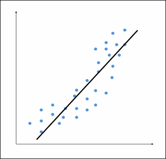
We can see that there is a natural curve to the pattern of datapoints. This linear model is unable to capture this. Let's see what a polynomial model would look like:

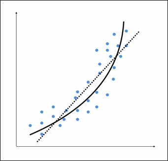
The dotted line represents the linear regression model, and the solid line represents the polynomial regression model. The curviness of this model is controlled by the degree of the polynomial. As the curviness of the model increases, it gets more accurate. However, curviness adds complexity to the model as well, hence, making it slower. This is a trade off where you have to decide between how accurate you want your model to be given the computational constraints.

How to do it…

Add the following lines to regressor.py:

from sklearn.preprocessing import PolynomialFeatures

polynomial = PolynomialFeatures(degree=3)

We initialized a polynomial of the degree 3 in the previous line. Now we have to represent the datapoints in terms of the coefficients of the polynomial:
```
X_train_transformed = polynomial.fit_transform(X_train)
```
Here, X_train_transformed represents the same input in the polynomial form.
Let's consider the first datapoint in our file and check whether it can predict the right output:
```
datapoint = [0.39,2.78,7.11]
poly_datapoint = polynomial.fit_transform(datapoint)

poly_linear_model = linear_model.LinearRegression()
poly_linear_model.fit(X_train_transformed, y_train)
print "\nLinear regression:", linear_regressor.predict(datapoint)[0]
print "\nPolynomial regression:", poly_linear_model.predict(poly_datapoint)[0]
```
The values in the variable datapoint are the values in the first line in the input data file. We are still fitting a linear regression model here. The only difference is in the way in which we represent the data. If you run this code, you will see the following output:
```
Linear regression: -11.0587294983
Polynomial regression: -10.9480782122
```
As you can see, this is close to the output value. If we want it to get closer, we need to increase the degree of the polynomial.

Let's make it 10 and see what happens:

polynomial = PolynomialFeatures(degree=10)

You should see something like the following:

Polynomial regression: -8.20472183853

Now, you can see that the predicted value is much closer to the actual output value.

Python Machine Learning Cookbook

By : Prateek Joshi, Vahid Mirjalili

Python Machine Learning Cookbook

By: Prateek Joshi, Vahid Mirjalili

Overview of this book

Related Content you might be interested in

Current Title:

Python Machine Learning Cookbook

Building a polynomial regressor

Getting ready

How to do it…