

Let's use a different regression method to solve the bicycle demand distribution problem. We will use the random forest regressor to estimate the output values. A random forest is a collection of decision trees. This basically uses a set of decision trees that are built using various subsets of the dataset, and then it uses averaging to improve the overall performance.
We will use the bike_day.csv file that is provided to you. This is also available at https://archive.ics.uci.edu/ml/datasets/Bike+Sharing+Dataset. There are 16 columns in this dataset. The first two columns correspond to the serial number and the actual date, so we won't use them for our analysis. The last three columns correspond to different types of outputs. The last column is just the sum of the values in the fourteenth and fifteenth columns, so we can leave these two out when we build our model.
Let's go ahead and see how to do this in Python. You have been provided with a file called bike_sharing.py that contains the full code. We will discuss the important parts of this, as follows:
We first need to import a couple of new packages, as follows:
import csv
from sklearn.ensemble import RandomForestRegressor
from housing import plot_feature_importances
We are processing a CSV file, so the CSV package is useful in handling these files. As it's a new dataset, we will have to define our own dataset loading function:
def load_dataset(filename):
    file_reader = csv.reader(open(filename, 'rb'), delimiter=',')
    X, y = [], []
    for row in file_reader:
        X.append(row[2:13])
        y.append(row[-1])

    # Extract feature names
    feature_names = np.array(X[0])

    # Remove the first row because they are feature names
    return np.array(X[1:]).astype(np.float32), np.array(y[1:]).astype(np.float32), feature_names
In this function, we just read all the data from the CSV file. The feature names are useful when we display it on a graph. We separate the data from the output values and return them.
Let's read the data and shuffle it to make it independent of the order in which the data is arranged in the file:
X, y, feature_names = load_dataset(sys.argv[1])
X, y = shuffle(X, y, random_state=7)
As we did earlier, we need to separate the data into training and testing. This time, let's use 90% of the data for training and the remaining 10% for testing:
num_training = int(0.9 * len(X))
X_train, y_train = X[:num_training], y[:num_training]
X_test, y_test = X[num_training:], y[num_training:]
Let's go ahead and train the regressor:
rf_regressor = RandomForestRegressor(n_estimators=1000, max_depth=10, min_samples_split=1)
rf_regressor.fit(X_train, y_train)
Here,
n_estimatorsrefers to the number of estimators, which is the number of decision trees that we want to use in our random forest. Themax_depthparameter refers to the maximum depth of each tree, and themin_samples_splitparameter refers to the number of data samples that are needed to split a node in the tree.Let's evaluate performance of the random forest regressor:
y_pred = rf_regressor.predict(X_test)
mse = mean_squared_error(y_test, y_pred)
evs = explained_variance_score(y_test, y_pred)
print "\n#### Random Forest regressor performance ####"
print "Mean squared error =", round(mse, 2)
print "Explained variance score =", round(evs, 2)
As we already have the function to plot the
importancesfeature, let's just call it directly:plot_feature_importances(rf_regressor.feature_importances_, 'Random Forest regressor', feature_names)
Once you run this code, you will see the following graph:
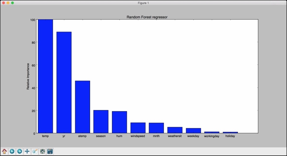
Looks like the temperature is the most important factor controlling the bicycle rentals.
Let's see what happens when you include fourteenth and fifteenth columns in the dataset. In the feature importance graph, every feature other than these two has to go to zero. The reason is that the output can be obtained by simply summing up the fourteenth and fifteenth columns, so the algorithm doesn't need any other features to compute the output. In the load_dataset function, make the following change inside the for loop:
X.append(row[2:15])
If you plot the feature importance graph now, you will see the following:
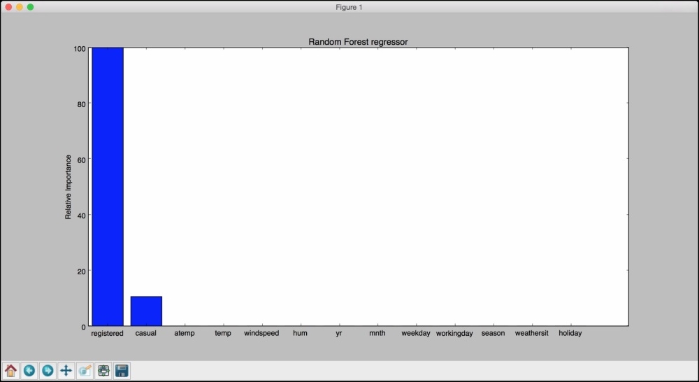
As expected, it says that only these two features are important. This makes sense intuitively because the final output is a simple summation of these two features. So, there is a direct relationship between these two variables and the output value. Hence, the regressor says that it doesn't need any other variable to predict the output. This is an extremely useful tool to eliminate redundant variables in your dataset.
There is another file called bike_hour.csv that contains data about how the bicycles are shared hourly. We need to consider columns 3 to 14, so let's make this change inside the load_dataset function:
X.append(row[2:14])
If you run this, you will see the performance of the regressor displayed, as follows:
#### Random Forest regressor performance ####
Mean squared error = 2619.87
Explained variance score = 0.92
The feature importance graph will look like the following:
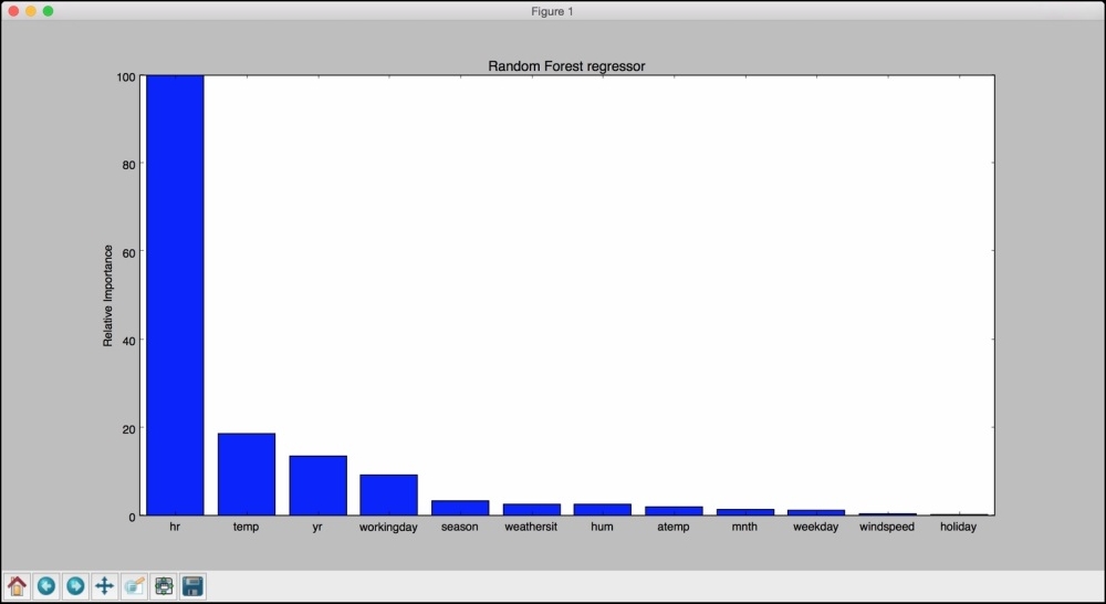
This shows that the hour of the day is the most important feature, which makes sense intuitively if you think about it! The next important feature is temperature, which is consistent with our earlier analysis.