Most of your analysis will make use of NumPy, even if you don’t use it explicitly. NumPy is an array manipulation library that is behind libraries such as pandas, Matplotlib, Biopython, and scikit-learn, among many others. While much of your bioinformatics work may not require explicit direct use of NumPy, you should be aware of its existence as it underpins almost everything you do, even if only indirectly via the other libraries.
In this recipe, we will use VAERS data to demonstrate how NumPy is behind many of the core libraries that we use. This is a very light introduction to the library so that you are aware that it exists and that it is behind almost everything. Our example will extract the number of cases from the five US states with more adverse effects, splitting them into age bins: 0 to 19 years, 20 to 39, up to 100 to 119.
Getting ready
Once again, we will be using the data from the first recipe, so make sure it’s available. The code for it can be found in Chapter02/NumPy.py.
How to do it…
Follow these steps:
- Let’s start by loading the data with pandas and reducing the data so that it’s related to the top five US states only:
import numpy as np
import pandas as pd
import matplotlib.pyplot as plt
vdata = pd.read_csv(
    "2021VAERSDATA.csv.gz", encoding="iso-8859-1")
vdata["STATE"] = vdata["STATE"].str.upper()
top_states = pd.DataFrame({
    "size": vdata.groupby("STATE").size().sort_values(ascending=False).head(5)}).reset_index()
top_states["rank"] = top_states.index
top_states = top_states.set_index("STATE")
top_vdata = vdata[vdata["STATE"].isin(top_states.index)]
top_vdata["state_code"] = top_vdata["STATE"].apply(
    lambda state: top_states["rank"].at[state]
).astype(np.uint8)
top_vdata = top_vdata[top_vdata["AGE_YRS"].notna()]
top_vdata.loc[:,"AGE_YRS"] = top_vdata["AGE_YRS"].astype(int)
top_states
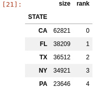
The top states are as follows. This rank will be used later to construct a NumPy matrix:
Figure 2.2 – US states with largest numbers of adverse effects
- Now, let’s extract the two NumPy arrays that contain age and state data:
age_state = top_vdata[["state_code", "AGE_YRS"]]
age_state["state_code"]
state_code_arr = age_state["state_code"].values
type(state_code_arr), state_code_arr.shape, state_code_arr.dtype
age_arr = age_state["AGE_YRS"].values
type(age_arr), age_arr.shape, age_arr.dtype
Note that the data that underlies pandas is NumPy data (the values call for both Series returns NumPy types). Also, you may recall that pandas has properties such as .shape or .dtype: these were inspired by NumPy and behave the same.
- Now, let’s create a NumPy matrix from scratch (a 2D array), where each row is a state and each column represents an age group:
age_state_mat = np.zeros((5,6), dtype=np.uint64)
for row in age_state.itertuples():
    age_state_mat[row.state_code, row.AGE_YRS//20] += 1
age_state_mat
The array has five rows – one for each state – and six columns – one for each age group. All the cells in the array must have the same type.
We initialize the array with zeros. There are many ways to initialize arrays, but if you have a very large array, initializing it may take a lot of time. Sometimes, depending on your task, it might be OK that the array is empty at the beginning (meaning it was initialized with random trash). In that case, using np.empty will be much faster. We use pandas iteration here: this is not the best way to do things from a pandas perspective, but we want to make the NumPy part very explicit.
- We can extract a single row – in our case, the data for a state – very easily. The same applies to a column. Let’s take California data and then the 0-19 age group:
cal = age_state_mat[0,:]
kids = age_state_mat[:,0]
Note the syntax to extract a row or a column. It should be familiar to you, given that pandas copied the syntax from NumPy and we encountered it in previous recipes.
- Now, let’s compute a new matrix where we have the fraction of cases per age group:
def compute_frac(arr_1d):
    return arr_1d / arr_1d.sum()
frac_age_stat_mat = np.apply_along_axis(compute_frac, 1, age_state_mat)
The last line applies the compute_frac function to all rows. compute_frac takes a single row and returns a new row where all the elements are divided by the total sum.
- Now, let’s create a new matrix that acts as a percentage instead of a fraction – simply because it reads better:
perc_age_stat_mat = frac_age_stat_mat * 100
perc_age_stat_mat = perc_age_stat_mat.astype(np.uint8)
perc_age_stat_mat
The first line simply multiplies all the elements of the 2D array by 100. Matplotlib is smart enough to traverse different array structures. That line will work if it’s presented with an array with any dimensions and would do exactly what is expected.
Here is the result:
Figure 2.3 – A matrix representing the distribution of vaccine-adverse effects in the five US states with the most cases
- Finally, let’s create a graphical representation of the matrix using Matplotlib:
fig = plt.figure()
ax = fig.add_subplot()
ax.matshow(perc_age_stat_mat, cmap=plt.get_cmap("Greys"))
ax.set_yticks(range(5))
ax.set_yticklabels(top_states.index)
ax.set_xticks(range(6))
ax.set_xticklabels(["0-19", "20-39", "40-59", "60-79", "80-99", "100-119"])
fig.savefig("matrix.png")
Do not dwell too much on the Matplotlib code – we are going to discuss it in the next recipe. The fundamental point here is that you can pass NumPy data structures to Matplotlib. Matplotlib, like pandas, is based on NumPy.
See also
The following is some extra information that may be useful:
- NumPy has many more features than the ones we’ve discussed here. There are plenty of books and tutorials on them. The official documentation is a good place to start: https://numpy.org/doc/stable/.
- There are many important issues to discover with NumPy, but probably one of the most important is broadcasting: NumPy’s ability to take arrays of different structures and get the operations right. For details, go to https://numpy.org/doc/stable/user/theory.broadcasting.html.


 Free Chapter


