
Let us first go through the deployment process, which is explained in the following sections. Bear in mind that this is not a unique architecture that can be deployed.
Deployment is a huge step in distinguishing all the OpenStack components that were covered previously. It confirms your understanding of how to start designing a complete OpenStack environment. Of course, assuming the versatility and flexibility of such a cloud management platform, OpenStack offers several possibilities that might be considered an advantage. However, on the other hand, you may face a challenge of taking the right design decision that suits your needs.
Basically, what you should consider in the first place is the responsibility in the Cloud. Depending on your cloud computing mission, it is essential to know what a coordinating IaaS is. The following are the use cases:
Apart from the knowledge of the aforementioned cloud service model providers, there are a few master keys that you should take into account in order to bring a well-defined architecture to a good basis that is ready to be deployed.
Though the system architecture design has evolved and is accompanied by the adoption of several methodology frameworks, many enterprises have successfully deployed OpenStack environments by going through a 3D process—a conceptual model design, logical model design, and physical model design.
It might be obvious that complexity increases from the conceptual to the logical design and from the logical to the physical design.
As the first conceptual phase, we will have a high-level reflection on what we will need from certain generic classes from the OpenStack architecture:
|
Class |
Role |
|---|---|
|
Compute |
Stores virtual machine images Provides a user interface |
|
Image |
Stores disk files Provides a user interface |
|
Object storage |
Provides a user interface |
|
Block storage |
Provides volumes Provides a user interface |
|
Network |
Provides network connectivity Provides a user interface |
|
Identity |
Provides authentication |
|
Dashboard |
Graphical user interface |
Let's map the generic basic classes in the following simplified diagram:
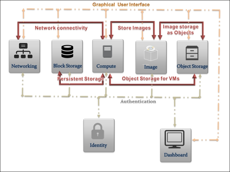
Keep in mind that the illustrated diagram will be refined over and over again since we will aim to integrate more services within our first basic design. In other words, we are following an incremental design approach within which we should exploit the flexibility of the OpenStack architecture.
At this level, we can have a vision and direction of the main goal without worrying about the details.
Based on the conceptual reflection phase, we are ready to construct the logical design. Most probably, you have a good idea about different OpenStack core components, which will be the basis of the formulation of the logical design that is done by laying down their logical representations.
Even though we have already taken the core of the OpenStack services component by component, you may need to map each of them to a logical solution within the complete design.
To do so, we will start by outlining the relations and dependencies between the services core of OpenStack. Most importantly, we aim to delve into the architectural level by keeping the details for the end. Thus, we will take into account the repartition of the OpenStack services between the new package services—the cloud controller and the compute node. You may wonder why such a consideration goes through a physical design classification. However, seeing the cloud controller and compute nodes as simple packages that encapsulate a bunch of OpenStack services, will help you refine your design at an early stage. Furthermore, this approach will plan in advance further high availability and scalability features, which allow you to introduce them later in more detail.
Note
Chapter 3, Learning OpenStack Clustering – Cloud Controllers and Compute Nodes, describes in depth how to distribute the OpenStack services between cloud controllers and compute nodes.
Thus, the physical model design will be elaborated based on the previous theoretical phases by assigning parameters and values to our design. Let's start with our first logical iteration:

Obviously, in a highly available setup, we should achieve a degree of redundancy in each service within OpenStack. You may wonder about the critical OpenStack services claimed in the first part of this chapter—the database and message queue. Why can't they be separately clustered or packaged on their own? This is a pertinent question. Remember that we are still in the second logical phase where we try to dive slowly and softly into the infrastructure without getting into the details. Besides, we keep on going from general to specific models, where we focus more on the generic details. Decoupling RabbitMQ or MySQL from now on may lead to your design being overlooked. Alternatively, you may risk skipping other generic design topics. On the other hand, preparing a generic logical design will help you to not stick to just one possible combination, since the future physical designs will rely on it.
Note
What about storage
The previous logical figure includes several essentials solutions for a high-scalable and redundant OpenStack environment such as virtual IP (VIP), HAProxy, and Pacemaker. The aforementioned technologies will be discussed in more detail in Chapter 6, Openstack HA and Failover.
Compute nodes are relatively simple as they are intended just to run the virtual machine's workload. In order to manage the VMs, the nova-compute service can be assigned for each compute node. Besides, we should not forget that the compute nodes will not be isolated; a Neutron agent and an optional Ceilometer compute agent may run this node.
You should now have a deeper understanding of the storage types within OpenStack—Swift and Cinder.
However, we did not cover a third-party software-defined storage called Ceph, which may combine or replace either or both of Swift and Cinder.
More details will be covered in Chapter 4, Learning OpenStack Storage – Deploying the Hybrid Storage Model. For now, we will design from a basic point where we have to decide how Cinder and/or Swift will be a part of our logical design.
Ultimately, a storage system becomes more complicated when it faces an exponential growth in the amount of data. Thus, the designing of your storage system is one of the critical steps that is required for a robust architecture.
Depending on your OpenStack business size environment, how much data do you need to store? Will your future PaaS construct a wide range of applications that run heavy-analysis data? What about the planned Environment as a Service (EaaS) model? Developers will need to incrementally back up their virtual machine's snapshots. We need persistent storage.
Don't put all your eggs in one basket. This is why we will include Cinder and Swift in the mission. Many thinkers will ask the following question: If one can be satisfied by ephemeral storage, why offer block storage? To answer this question, you may think about ephemeral storage as the place where the end user will not be able to access the virtual disk associated with its VM when it is terminated. Ephemeral storage should mainly be used in production that takes place in a high-scale environment, where users are actively concerned about their data, VM, or application. If you plan that your storage design should be 100 percent persistent, backing up everything wisely will make you feel better. This helps you figure out the best way to store data that grows exponentially by using specific techniques that allow them to be made available at any time. Remember that the current design applies for medium to large infrastructures. Ephemeral storage can also be a choice for certain users, for example, when they consider building a test environment. Considering the same case for Swift, we have claimed previously that the object storage might be used to store machine images, but when is this the case?
Simply, when you provide the extra hardware that fulfils certain Swift requirements: replication and redundancy.
Running a wide production environment while storing machine images on the local file system is not really good practice. First, the image can be accessed by different services and requested by thousands of users at a time. No wonder the controller is already exhausted by the forwarding and routing of the requests between the different APIs in addition to the computation of each resources through disk I/O, memory, and CPU. Each request will cause performance degradation, but it will not fail! Keeping an image in a filesystem under a heavy load will certainly bring the controller to a high latency and it may fail.
Henceforth, we might consider loosely coupled models, where the storage with a specific performance is considered a best fit for the production environment.
Thus, Swift will be used to store images, while Cinder will be used for persistent volumes for virtual machines (check the Swift controller node):

Obviously, Cinder LVM does not provide any redundancy capability between the Cinder LVM nodes. Losing the data in a Cinder LVM node is a disaster. You may want to perform a backup for each node. This can be helpful, but it will be a very tedious task! Let's design for resiliency. We have put what's necessary on the table. Now, what we need is a glue!
One of the most complicated system designing steps is the part concerning the network! Now, let's look under the hood to see how all the different services that were defined previously should be connected.
OpenStack shows a wide range of networking configurations that vary between the basic and complicated. Terms such as Open vSwitch, Neutron coupled with the VLAN segmentation, and VMware NSX with Neutron are not intuitively obvious from their appearance to be able to be implemented without fetching their use case in our design. Thus, this important step implies that you may differ between different network topologies because of the reasons behind why every choice was made and why it may work for a given use case.
OpenStack has moved from simplistic network features to complicated features, but of course there is a reason—more flexibility! This is why OpenStack is here. It brings as much flexibility as it can! Without taking any random network-related decisions, let's see which network modes are available. We will keep on filtering until we hit the first correct target topology:
|
Network mode |
Network specification |
Implementation |
|---|---|---|
|
Nova-network |
Flat network design without VMs grouping or isolation |
Nova-network FlatDHCP |
|
Multiple tenants and VMs Predefined fixed private IP space size |
Nova-network VLANManager | |
|
Neutron |
Multiple tenants and VMs Predefined switches and routers configuration |
Neutron VLAN |
|
Increased tenants and VM groups Lower performance |
Neutron GRE |
The preceding table shows a simple differentiation between two different logical network designs for OpenStack. Every mode shows its own requirements, which is very important and should be taken into consideration before the deployment.
Arguing about our example choice, since we aim to deploy a very flexible large-scale environment, we will toggle the Neutron choice for networking management instead of the nova-network.
Note that it is also possible to keep on going with nova-network, but you have to worry about SPOF. Since the nova-network service can run on a single node (cloud controller) next to other network services such as DHCP and DNS, it is required in this case to implement your nova-network service in a multihost networking model, where cloning such a service in every compute node will save you from a bottleneck scenario. In addition, the choice was made for Neutron, since we started from a basic network deployment. We will cover more advanced features in the subsequent chapters of this book.
We would like to exploit a major advantage of Neutron compared to the nova-network, which is the virtualization of layers 2 and 3 of the OSI network model.
Remember that Neutron will enable us to support more subnets per private network segment. Based on Open vSwitch, you will discover that Neutron is becoming a vast network technology.
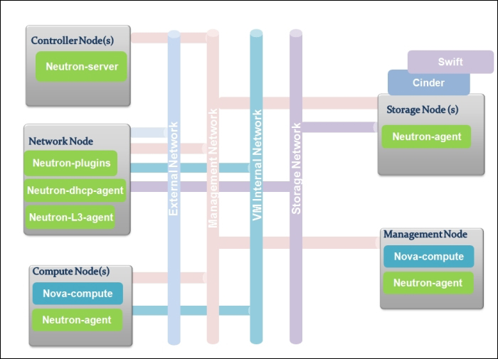
Let's see how we can expose our logical network design. For performance reasons, it is highly recommended to implement a topology that can handle different types of traffic by using separated logical networks.
In this way, as your network grows, it will still be manageable in case a sudden bottleneck or an unexpected failure affects a segment.
Let us look at the different networks that are needed to operate the OpenStack environment.
The features of an external or a public network are as follows:
Global connectivity
It performs SNAT from the VM instances that run on the compute node to the Internet for floating IPs
Note
SNAT refers to Source Network Address Translation. It allows traffic from a private network to go out to the Internet. OpenStack supports SNAT through its Neutron APIs for routers. More information can be found at http://en.wikipedia.org/wiki/Network_address_translation.
It provides connection to the controller nodes in order to access the OpenStack interfaces
It provides virtual IPs (VIPs) for public endpoints that are used to connect the OpenStack services APIs
It provides a connection to the external services that need to be public, such as an access to the Zabbix monitoring system
The main feature of a storage network is that it separates the storage traffic by means of a VLAN isolation.
An orchestrator node was not described previously since it is not a native OpenStack service. Different nodes need to get IP addresses, the DNS, and the DHCP service where the Orchestrator node comes into play. You should also keep in mind that in a large environment, you will need a node provisioning technique which your nodes will be configured to boot, by using PXE and TFTP.
Thus, the management network will act as an Orchestrator data network that provides the following:
Administrative networking tasks
OpenStack services communication
Separate HA traffic
The features of the internal virtual machine network are as follows:
Private network between virtual machines
Nonroutable IPs
Closed network between the virtual machines and the network L3 nodes, routing to the Internet, and the floating IPs backwards to the VMs
For the sake of simplicity, we will not go into the details of, for instance, the Neutron VLAN segmentation.
The next step is to validate our network design in a simple diagram:
Finally, we will bring our logical design to life in the form of a physical design. At this stage, we need to assign parameters. The physical design encloses all the components that we dealt with previously in the logical design. Of course, you will appreciate how such an escalation in the design breaks down the complexity of the OpenStack environment and helps us distinguish between the types of hardware specifications that you will need.
We can start with a limited number of servers just to set the first deployment of our environment effectively. First, we will consider a small production environment that is highly scalable and extensible. This is what we have covered previously—expecting a sudden growth and being ready for an exponentially increasing number of requests to service instances.
You have to consider the fact that the hardware commodity selection will accomplish the mission of our massive scalable architecture.
Since the architecture is being designed to scale horizontally, a commodity cost-effective hardware can be used.
In order to expect our infrastructure economy, it would be great to make some basic hardware calculations for the first estimation of our exact requirements.
Considering the possibility of experiencing contentions for resources such as CPU, RAM, network, and disk, you cannot wait for a particular physical component to fail before you take corrective action, which might be more complicated.
Let's inspect a real-life example of the impact of underestimating capacity planning. A Cloud-hosting company set up two medium servers, one for an e-mail server, and the other to host the official website. The company, which is one of our several clients, grew in a few months and eventually, we ran out of disk space. We expected such an issue to get resolved in a few hours, but it took days. The problem was that all the parties did not make proper use of the "cloud", which points to the "on demand" way. The issue had been serious for both the parties. The e-mail server, which is one of the most critical aspects of a company, had been overloaded and the Mean Time To Repair (MTTR) was increasing exponentially. The Cloud provider did not expect this!
Well, it might be ridiculous to write down your SLA report and describe in your incident management section the reason—we did not expect such growth! Later, after redeploying the virtual machine with more disk space, the e-mail server would irritate everyone in the company with a message saying, "We can authenticate but our e-mails are not being sent! They are queued!" The other guy claimed, "Finally, I have sent an e-mail 2 hours ago and I got a phone call that is received." Unfortunately, the cloud paradigm was designed to avoid such scenarios and bring more success factors that can be achieved by hosting providers. Capacity management is considered a day-to-day responsibility where you have to stay updated with regard to software or hardware upgrades.
Through a continuous monitoring process of service consumption, you will be able to reduce the IT risk and provide a quick response to the customer's needs.
From your first hardware deployment, keep running your capacity management processes by looping through tuning, monitoring, and analysis.
The next stop will take into account your tuned parameters and introduce within your hardware/software the right change, which involves a synergy of the change management process.
Let's make our first calculation based on certain requirements. We aim to run 200 VMs in our OpenStack environment.
The following are the calculation-related assumptions:
200 virtual machines
No CPU oversubscribing
Number of GHz per core: 2.6 GHz
Hyper-threading supported: use factor 2
Number of GHz per VM (AVG compute units) = 2 GHz
Number of GHz per VM (MAX compute units) = 16 GHz
Intel Xeon E5-2648L v2 core CPU = 10
CPU sockets per server = 2
Number of CPU cores per virtual machine:
16 / (2.6 * 2) = 3.076
We need to assign at least 3 CPU cores per VM.
The formula for its calculation will be as follows: max GHz /(number of GHz per core x 1.3 for hyper-threading)
Total number of CPU cores:
(200 * 2) / 2.6 = 153.846
We have 153 CPU cores for 200 VMs.
The formula for calculation will be as follows:
(number of VMs x number of GHz per VM) / number of GHz per core
Number of core CPU sockets:
153 / 10 = 15.3
The formula for calculation will be as follows:
Total number of sockets / number of sockets per server
Number of socket servers:
15 / 2 = 7.5
You will need around 7 to 8 dual socket servers.
The formula for calculation will be as follows:
Total number of sockets / Number of sockets per server
The number of virtual machines per server with 8 dual socket servers will be calculated as follows:
200 / 8 = 25
The formula for calculation will be as follows:
Number of virtual machines / number of servers
We can deploy 25 virtual machines per server.
Based on the previous example, 25 VMs can be deployed per compute node. Memory sizing is also important to avoid making unreasonable resource allocations.
Let's make an assumption list:
2 GB RAM per VM
8 GB RAM maximum dynamic allocation per VM
Compute nodes supporting slots of: 2, 4, 8, and 16 GB sticks
Keep in mind that it always depends on your budget and needs
RAM available per compute node:
8 * 25 = 200 GB
Considering the number of sticks supported by your server, you will need around 256 GB installed. Therefore, the total number of RAM sticks installed can be calculated in the following way:
256 / 16 = 16
The formula for calculation is as follows:
Total available RAM / MAX Available RAM-Stick size
To fulfill the plans that were drawn for the network previously, we need to achieve the best performance and networking experience. Let's have a look at our assumptions:
200 Mbits/second is needed per VM
Minimum network latency
To do this, it might be possible to serve our VMs by using a 10 GB link for each server, which will give:
10000 Mbits/second / 25VMs = 400 Mbits/second
This is a very satisfying value. We need to consider another factor—highly available network architecture. Thus, an alternative is using two data switches with a minimum of 24 ports for data.
Thinking about growth from now, two 48-port switches will be in place.
What about the growth of the rack size? In this case, you should think about the example of switch aggregation that uses the Virtual Link Trunking (VLT) technology between the switches in the aggregation. This feature allows each server rack to divide their links between the pair of switches to achieve a powerful active-active forwarding while using the full bandwidth capability with no requirement for a spanning tree.
Considering the previous example, you need to plan for an initial storage capacity per server that will serve 25 VMs each.
Let's make the following assumptions:
The usage of ephemeral storage for a local drive for the VM
100 GB for storage for each VM's drive
The usage of persistent storage for remote attaching volumes to VMs
A simple calculation we provide for 200 VMs a space of 200*100 = 20 TB of local storage.
You can assign 250 GB of persistent storage per VM to have 200*200 = 40 TB of persistent storage.
Therefore, we can conclude how much storage should be installed by the server serving 20 VMs 150*25 = 3.5 TB of storage on the server.
If you plan to include object storage as we mentioned earlier, we can assume that we will need 25 TB of object storage.
Most probably, you have an idea about the replication of object storage in OpenStack, which implies the usage of three times the required space for replication.
In other words, you should consider that the planning of X TB for object storage will be multiplied by three automatically based on our assumption; 25*3 = 75 TB.
Also, if you consider an object storage based on zoning, you will have to accommodate at least five times the needed space. This means; 25 * 5 = 125 TB.
Other considerations, such as the best storage performance using SSD, can be useful for a better throughput where you can invest more boxes to get an increased IOPS.
For example, working with SSD with 20K IOPS installed in a server with eight slot drives will bring you:
(20K * 8) / 25 = 6.4 K Read IOPS and 3.2K Write IOPS
That is not bad for a production starter!
What about best practices? Is it just a theory? Does anyone adhere to such formulas? Well, let's bring some best practices under the microscope by exposing the OpenStack design flavor.
In a typical OpenStack production environment, the minimum requirement for disk space per compute node is 300 GB with a minimum RAM of 128 GB and a dual 8-core CPUs.
Let's imagine a scenario where, due to budget limitations, you start your first compute node with costly hardware that has a 600 GB disk space, 16-core CPUs, and 256 GB of RAM.
Assuming that your OpenStack environment continues to grow, you may decide to purchase more hardware—a big one at an incredible price! A second compute instance is placed to scale up.
Shortly after this, you may find out that the demand is increasing. You may start splitting requests into different compute nodes but keep on continuing scaling up with the hardware. At some point, you will be alerted to reaching your budget limit!
There are certainly times when the best practices aren't in fact the best for your design. The previous example illustrated a commonly overlooked requirement for the OpenStack deployment.
If the minimal hardware requirement is strictly followed, it may result in an exponential cost with regard to the hardware expenses, especially for new project starters.
Thus, you may choose what exactly works for you and consider the constraints that exist in your environment.
Keep in mind that the best practices are a user manual or a guideline; apply them when you find what you need to be deployed and how it should be set up.
On the other hand, do not stick to values, but stick to rules. Let's bring the previous example under the microscope again—scaling up shows more risk that may lead to failure than scaling out or horizontally. The reason behind such a design is to allow for a fast scale of transactions at the cost of a duplicated compute functionality and smaller systems at a lower cost.
Transactions and requests in the compute node may grow tremendously in a short time to a point that a single big compute node with 16 core CPUs starts failing performance wise, while a few small compute nodes with 4 core CPUs can proceed to complete the job successfully.