
In this chapter, we will take a tour through a selection of popular and powerful machine learning algorithms that are commonly used in academia as well as in the industry. While learning about the differences between several supervised learning algorithms for classification, we will also develop an intuitive appreciation of their individual strengths and weaknesses. Also, we will take our first steps with the scikit-learn library, which offers a user-friendly interface for using those algorithms efficiently and productively.
The topics that we will learn about throughout this chapter are as follows:
- Introduction to the concepts of popular classification algorithms
- Using the scikit-learn machine learning library
- Questions to ask when selecting a machine learning algorithm
Choosing an appropriate classification algorithm for a particular problem task requires practice: each algorithm has its own quirks and is based on certain assumptions. To restate the "No Free Lunch" theorem: no single classifier works best across all possible scenarios. In practice, it is always recommended that you compare the performance of at least a handful of different learning algorithms to select the best model for the particular problem; these may differ in the number of features or samples, the amount of noise in a dataset, and whether the classes are linearly separable or not.
Eventually, the performance of a classifier, computational power as well as predictive power, depends heavily on the underlying data that are available for learning. The five main steps that are involved in training a machine learning algorithm can be summarized as follows:
- Selection of features.
- Choosing a performance metric.
- Choosing a classifier and optimization algorithm.
- Evaluating the performance of the model.
- Tuning the algorithm.
Since the approach of this book is to build machine learning knowledge step by step, we will mainly focus on the principal concepts of the different algorithms in this chapter and revisit topics such as feature selection and preprocessing, performance metrics, and hyperparameter tuning for more detailed discussions later in this book.
In Chapter 2, Training Machine Learning Algorithms for Classification, you learned about two related learning algorithms for classification: the perceptron rule and Adaline, which we implemented in Python by ourselves. Now we will take a look at the scikit-learn API, which combines a user-friendly interface with a highly optimized implementation of several classification algorithms. However, the scikit-learn library offers not only a large variety of learning algorithms, but also many convenient functions to preprocess data and to fine-tune and evaluate our models. We will discuss this in more detail together with the underlying concepts in Chapter 4, Building Good Training Sets – Data Preprocessing, and Chapter 5, Compressing Data via Dimensionality Reduction.
To get started with the scikit-learn library, we will train a perceptron model similar to the one that we implemented in Chapter 2, Training Machine Learning Algorithms for Classification. For simplicity, we will use the already familiar Iris dataset throughout the following sections. Conveniently, the Iris dataset is already available via scikit-learn, since it is a simple yet popular dataset that is frequently used for testing and experimenting with algorithms. Also, we will only use two features from the Iris flower dataset for visualization purposes.
We will assign the petal length and petal width of the 150 flower samples to the feature matrix X and the corresponding class labels of the flower species to the vector y:
>>> from sklearn import datasets >>> import numpy as np >>> iris = datasets.load_iris() >>> X = iris.data[:, [2, 3]] >>> y = iris.target
If we executed np.unique(y) to return the different class labels stored in iris.target, we would see that the Iris flower class names, Iris-Setosa, Iris-Versicolor, and Iris-Virginica, are already stored as integers (0, 1, 2), which is recommended for the optimal performance of many machine learning libraries.
To evaluate how well a trained model performs on unseen data, we will further split the dataset into separate training and test datasets. Later in Chapter 5, Compressing Data via Dimensionality Reduction, we will discuss the best practices around model evaluation in more detail:
>>> from sklearn.cross_validation import train_test_split >>> X_train, X_test, y_train, y_test = train_test_split( ... X, y, test_size=0.3, random_state=0)
Using the train_test_split function from scikit-learn's cross_validation module, we randomly split the X and y arrays into 30 percent test data (45 samples) and 70 percent training data (105 samples).
Many machine learning and optimization algorithms also require feature scaling for optimal performance, as we remember from the
gradient descent example in Chapter 2, Training Machine Learning Algorithms for Classification. Here, we will standardize the features using the StandardScaler class from scikit-learn's preprocessing module:
>>> from sklearn.preprocessing import StandardScaler >>> sc = StandardScaler() >>> sc.fit(X_train) >>> X_train_std = sc.transform(X_train) >>> X_test_std = sc.transform(X_test)
Using the preceding code, we loaded the StandardScaler class from the preprocessing module and initialized a new StandardScaler object that we assigned to the variable sc. Using the fit method, StandardScaler estimated the parameters  (sample mean) and
  (standard deviation) for each feature dimension from the training data. By calling the
 transform method, we then standardized the training data using those estimated parameters and . Note that we used the same scaling parameters to standardize the test set so that both the values in the training and test dataset are comparable to each other.
Having standardized the training data, we can now train a perceptron model. Most algorithms in scikit-learn already support multiclass classification by default via the One-vs.-Rest (OvR) method, which allows us to feed the three flower classes to the perceptron all at once. The code is as follows:
>>> from sklearn.linear_model import Perceptron >>> ppn = Perceptron(n_iter=40, eta0=0.1, random_state=0) >>> ppn.fit(X_train_std, y_train)
The scikit-learn interface reminds us of our perceptron implementation in Chapter 2, Training Machine Learning Algorithms for Classification: after loading the Perceptron class from the linear_model module, we initialized a new Perceptron object and trained the model via the fit method. Here, the model parameter eta0 is equivalent to the learning rate eta that we used in our own perceptron implementation, and the parameter n_iter defines the number of epochs (passes over the training set). As we remember from Chapter 2, Training Machine Learning Algorithms for Classification, finding an appropriate learning rate requires some experimentation. If the learning rate is too large, the algorithm will overshoot the global cost minimum. If the learning rate is too small, the algorithm requires more epochs until convergence, which can make the learning slow—especially for large datasets. Also, we used the random_state parameter for reproducibility of the initial shuffling of the training dataset after each epoch.
Having trained a model in scikit-learn, we can make predictions via the predict method, just like in our own perceptron implementation in Chapter 2, Training Machine Learning Algorithms for Classification. The code is as follows:
>>> y_pred = ppn.predict(X_test_std)
>>> print('Misclassified samples: %d' % (y_test != y_pred).sum())
Misclassified samples: 4On executing the preceding code, we see that the perceptron misclassifies 4 out of the 45 flower samples. Thus, the misclassification error on the test dataset is 0.089 or 8.9 percent  .
.
Scikit-learn also implements a large variety of different performance metrics that are available via the metrics module. For example, we can calculate the classification accuracy of the perceptron on the test set as follows:
>>> from sklearn.metrics import accuracy_score
>>> print('Accuracy: %.2f' % accuracy_score(y_test, y_pred))
0.91Here, y_test are the true class labels and y_pred are the class labels that we predicted previously.
Note
Note that we evaluate the performance of our models based on the test set in this chapter. In Chapter 5, Compressing Data via Dimensionality Reduction, you will learn about useful techniques, including graphical analysis such as learning curves, to detect and prevent overfitting. Overfitting means that the model captures the patterns in the training data well, but fails to generalize well to unseen data.
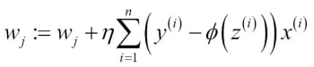
Finally, we can use our plot_decision_regions function from Chapter 2, Training Machine Learning Algorithms for Classification, to plot the
decision regions of our newly trained perceptron model and visualize how well it separates the different flower samples. However, let's add a small modification to highlight the samples from the test dataset via small circles:
from matplotlib.colors import ListedColormap
import matplotlib.pyplot as plt
def plot_decision_regions(X, y, classifier,
test_idx=None, resolution=0.02):
# setup marker generator and color map
markers = ('s', 'x', 'o', '^', 'v')
colors = ('red', 'blue', 'lightgreen', 'gray', 'cyan')
cmap = ListedColormap(colors[:len(np.unique(y))])
# plot the decision surface
x1_min, x1_max = X[:, 0].min() - 1, X[:, 0].max() + 1
x2_min, x2_max = X[:, 1].min() - 1, X[:, 1].max() + 1
xx1, xx2 = np.meshgrid(np.arange(x1_min, x1_max, resolution),
np.arange(x2_min, x2_max, resolution))
Z = classifier.predict(np.array([xx1.ravel(), xx2.ravel()]).T)
Z = Z.reshape(xx1.shape)
plt.contourf(xx1, xx2, Z, alpha=0.4, cmap=cmap)
plt.xlim(xx1.min(), xx1.max())
plt.ylim(xx2.min(), xx2.max())
# plot all samples
X_test, y_test = X[test_idx, :], y[test_idx]
for idx, cl in enumerate(np.unique(y)):
plt.scatter(x=X[y == cl, 0], y=X[y == cl, 1],
alpha=0.8, c=cmap(idx),
marker=markers[idx], label=cl)
# highlight test samples
if test_idx:
X_test, y_test = X[test_idx, :], y[test_idx]
plt.scatter(X_test[:, 0], X_test[:, 1], c='',
alpha=1.0, linewidth=1, marker='o',
s=55, label='test set')With the slight modification that we made to the plot_decision_regions function (highlighted in the preceding code), we can now specify the indices of the samples that we want to mark on the resulting plots. The code is as follows:
>>> X_combined_std = np.vstack((X_train_std, X_test_std))
>>> y_combined = np.hstack((y_train, y_test))
>>> plot_decision_regions(X=X_combined_std,
... y=y_combined,
... classifier=ppn,
... test_idx=range(105,150))
>>> plt.xlabel('petal length [standardized]')
>>> plt.ylabel('petal width [standardized]')
>>> plt.legend(loc='upper left')
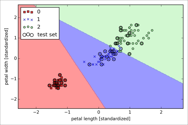
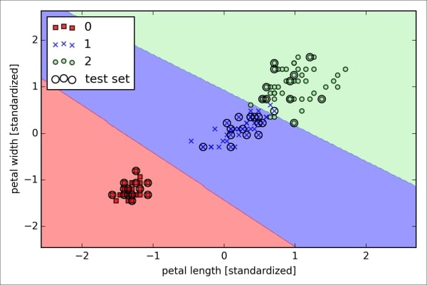
>>> plt.show()As we can see in the resulting plot, the three flower classes cannot be perfectly separated by a linear decision boundaries:
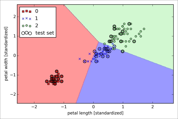
We remember from our discussion in Chapter 2, Training Machine Learning Algorithms for Classification, that the perceptron algorithm never converges on datasets that aren't perfectly linearly separable, which is why the use of the perceptron algorithm is typically not recommended in practice. In the following sections, we will look at more powerful linear classifiers that converge to a cost minimum even if the classes are not perfectly linearly separable.
Note
The Perceptron as well as other scikit-learn functions and classes have additional parameters that we omit for clarity. You can read more about those parameters using the help function in Python (for example, help(Perceptron)) or by going through the excellent scikit-learn online documentation at http://scikit-learn.org/stable/.
Training a perceptron via scikit-learn
To get started with the scikit-learn library, we will train a perceptron model similar to the one that we implemented in Chapter 2, Training Machine Learning Algorithms for Classification. For simplicity, we will use the already familiar Iris dataset throughout the following sections. Conveniently, the Iris dataset is already available via scikit-learn, since it is a simple yet popular dataset that is frequently used for testing and experimenting with algorithms. Also, we will only use two features from the Iris flower dataset for visualization purposes.
We will assign the petal length and petal width of the 150 flower samples to the feature matrix X and the corresponding class labels of the flower species to the vector y:
>>> from sklearn import datasets >>> import numpy as np >>> iris = datasets.load_iris() >>> X = iris.data[:, [2, 3]] >>> y = iris.target
If we executed np.unique(y) to return the different class labels stored in iris.target, we would see that the Iris flower class names, Iris-Setosa, Iris-Versicolor, and Iris-Virginica, are already stored as integers (0, 1, 2), which is recommended for the optimal performance of many machine learning libraries.
To evaluate how well a trained model performs on unseen data, we will further split the dataset into separate training and test datasets. Later in Chapter 5, Compressing Data via Dimensionality Reduction, we will discuss the best practices around model evaluation in more detail:
>>> from sklearn.cross_validation import train_test_split >>> X_train, X_test, y_train, y_test = train_test_split( ... X, y, test_size=0.3, random_state=0)
Using the train_test_split function from scikit-learn's cross_validation module, we randomly split the X and y arrays into 30 percent test data (45 samples) and 70 percent training data (105 samples).
Many machine learning and optimization algorithms also require feature scaling for optimal performance, as we remember from the
gradient descent example in Chapter 2, Training Machine Learning Algorithms for Classification. Here, we will standardize the features using the StandardScaler class from scikit-learn's preprocessing module:
>>> from sklearn.preprocessing import StandardScaler >>> sc = StandardScaler() >>> sc.fit(X_train) >>> X_train_std = sc.transform(X_train) >>> X_test_std = sc.transform(X_test)
Using the preceding code, we loaded the StandardScaler class from the preprocessing module and initialized a new StandardScaler object that we assigned to the variable sc. Using the fit method, StandardScaler estimated the parameters (sample mean) and (standard deviation) for each feature dimension from the training data. By calling the transform method, we then standardized the training data using those estimated parameters and . Note that we used the same scaling parameters to standardize the test set so that both the values in the training and test dataset are comparable to each other.
Having standardized the training data, we can now train a perceptron model. Most algorithms in scikit-learn already support multiclass classification by default via the One-vs.-Rest (OvR) method, which allows us to feed the three flower classes to the perceptron all at once. The code is as follows:
>>> from sklearn.linear_model import Perceptron >>> ppn = Perceptron(n_iter=40, eta0=0.1, random_state=0) >>> ppn.fit(X_train_std, y_train)
The scikit-learn interface reminds us of our perceptron implementation in Chapter 2, Training Machine Learning Algorithms for Classification: after loading the Perceptron class from the linear_model module, we initialized a new Perceptron object and trained the model via the fit method. Here, the model parameter eta0 is equivalent to the learning rate eta that we used in our own perceptron implementation, and the parameter n_iter defines the number of epochs (passes over the training set). As we remember from Chapter 2, Training Machine Learning Algorithms for Classification, finding an appropriate learning rate requires some experimentation. If the learning rate is too large, the algorithm will overshoot the global cost minimum. If the learning rate is too small, the algorithm requires more epochs until convergence, which can make the learning slow—especially for large datasets. Also, we used the random_state parameter for reproducibility of the initial shuffling of the training dataset after each epoch.
Having trained a model in scikit-learn, we can make predictions via the predict method, just like in our own perceptron implementation in Chapter 2, Training Machine Learning Algorithms for Classification. The code is as follows:
>>> y_pred = ppn.predict(X_test_std)
>>> print('Misclassified samples: %d' % (y_test != y_pred).sum())
Misclassified samples: 4On executing the preceding code, we see that the perceptron misclassifies 4 out of the 45 flower samples. Thus, the misclassification error on the test dataset is 0.089 or 8.9 percent .
Scikit-learn also implements a large variety of different performance metrics that are available via the metrics module. For example, we can calculate the classification accuracy of the perceptron on the test set as follows:
>>> from sklearn.metrics import accuracy_score
>>> print('Accuracy: %.2f' % accuracy_score(y_test, y_pred))
0.91Here, y_test are the true class labels and y_pred are the class labels that we predicted previously.
Note
Note that we evaluate the performance of our models based on the test set in this chapter. In Chapter 5, Compressing Data via Dimensionality Reduction, you will learn about useful techniques, including graphical analysis such as learning curves, to detect and prevent overfitting. Overfitting means that the model captures the patterns in the training data well, but fails to generalize well to unseen data.
Finally, we can use our plot_decision_regions function from Chapter 2, Training Machine Learning Algorithms for Classification, to plot the
decision regions of our newly trained perceptron model and visualize how well it separates the different flower samples. However, let's add a small modification to highlight the samples from the test dataset via small circles:
from matplotlib.colors import ListedColormap
import matplotlib.pyplot as plt
def plot_decision_regions(X, y, classifier,
test_idx=None, resolution=0.02):
# setup marker generator and color map
markers = ('s', 'x', 'o', '^', 'v')
colors = ('red', 'blue', 'lightgreen', 'gray', 'cyan')
cmap = ListedColormap(colors[:len(np.unique(y))])
# plot the decision surface
x1_min, x1_max = X[:, 0].min() - 1, X[:, 0].max() + 1
x2_min, x2_max = X[:, 1].min() - 1, X[:, 1].max() + 1
xx1, xx2 = np.meshgrid(np.arange(x1_min, x1_max, resolution),
np.arange(x2_min, x2_max, resolution))
Z = classifier.predict(np.array([xx1.ravel(), xx2.ravel()]).T)
Z = Z.reshape(xx1.shape)
plt.contourf(xx1, xx2, Z, alpha=0.4, cmap=cmap)
plt.xlim(xx1.min(), xx1.max())
plt.ylim(xx2.min(), xx2.max())
# plot all samples
X_test, y_test = X[test_idx, :], y[test_idx]
for idx, cl in enumerate(np.unique(y)):
plt.scatter(x=X[y == cl, 0], y=X[y == cl, 1],
alpha=0.8, c=cmap(idx),
marker=markers[idx], label=cl)
# highlight test samples
if test_idx:
X_test, y_test = X[test_idx, :], y[test_idx]
plt.scatter(X_test[:, 0], X_test[:, 1], c='',
alpha=1.0, linewidth=1, marker='o',
s=55, label='test set')With the slight modification that we made to the plot_decision_regions function (highlighted in the preceding code), we can now specify the indices of the samples that we want to mark on the resulting plots. The code is as follows:
>>> X_combined_std = np.vstack((X_train_std, X_test_std))
>>> y_combined = np.hstack((y_train, y_test))
>>> plot_decision_regions(X=X_combined_std,
... y=y_combined,
... classifier=ppn,
... test_idx=range(105,150))
>>> plt.xlabel('petal length [standardized]')
>>> plt.ylabel('petal width [standardized]')
>>> plt.legend(loc='upper left')
>>> plt.show()As we can see in the resulting plot, the three flower classes cannot be perfectly separated by a linear decision boundaries:
We remember from our discussion in Chapter 2, Training Machine Learning Algorithms for Classification, that the perceptron algorithm never converges on datasets that aren't perfectly linearly separable, which is why the use of the perceptron algorithm is typically not recommended in practice. In the following sections, we will look at more powerful linear classifiers that converge to a cost minimum even if the classes are not perfectly linearly separable.
Note
The Perceptron as well as other scikit-learn functions and classes have additional parameters that we omit for clarity. You can read more about those parameters using the help function in Python (for example, help(Perceptron)) or by going through the excellent scikit-learn online documentation at http://scikit-learn.org/stable/.
Although the perceptron rule offers a nice and easygoing introduction to machine learning algorithms for classification, its biggest disadvantage is that it never converges if the classes are not perfectly linearly separable. The classification task in the previous section would be an example of such a scenario. Intuitively, we can think of the reason as the weights are continuously being updated since there is always at least one misclassified sample present in each epoch. Of course, you can change the learning rate and increase the number of epochs, but be warned that the perceptron will never converge on this dataset. To make better use of our time, we will now take a look at another simple yet more powerful algorithm for linear and binary classification problems: logistic regression. Note that, in spite of its name, logistic regression is a model for classification, not regression.
Logistic regression is a classification model that is very easy to implement but performs very well on linearly separable classes. It is one of the most widely used algorithms for classification in industry. Similar to the perceptron and Adaline, the logistic regression model in this chapter is also a linear model for binary classification that can be extended to multiclass classification via the OvR technique.
To explain the idea behind logistic regression as a probabilistic model, let's first introduce the
odds ratio, which is the odds in favor of a particular event. The odds ratio can be written as  , where
  stands for the probability of the positive event. The term positive event does not necessarily mean good, but refers to the event that we want to predict, for example, the probability that a patient has a certain disease; we can think of the positive event as class label
  . We can then further define the
logit function, which is simply the logarithm of the odds ratio (log-odds):
. We can then further define the
logit function, which is simply the logarithm of the odds ratio (log-odds):
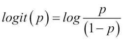
The logit function takes input values in the range 0 to 1 and transforms them to values over the entire real number range, which we can use to express a linear relationship between feature values and the log-odds:
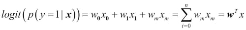
Here,  is the conditional probability that a particular sample belongs to class 1 given its features x.
Now what we are actually interested in is predicting the probability that a certain sample belongs to a particular class, which is the inverse form of the logit function. It is also called the logistic function, sometimes simply abbreviated as sigmoid function due to its characteristic S-shape.
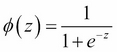
Here, z is the net input, that is, the linear combination of weights and sample features and can be calculated as  .
.
Now let's simply plot the sigmoid function for some values in the range -7 to 7 to see what it looks like:
>>> import matplotlib.pyplot as plt
>>> import numpy as np
>>> def sigmoid(z):
... return 1.0 / (1.0 + np.exp(-z))
>>> z = np.arange(-7, 7, 0.1)
>>> phi_z = sigmoid(z)
>>> plt.plot(z, phi_z)
>>> plt.axvline(0.0, color='k')
>>> plt.axhspan(0.0, 1.0, facecolor='1.0', alpha=1.0, ls='dotted')
>>> plt.axhline(y=0.5, ls='dotted', color='k')
>>> plt.yticks([0.0, 0.5, 1.0])
>>> plt.ylim(-0.1, 1.1)
>>> plt.xlabel('z')
>>> plt.ylabel('$\phi (z)$')
>>> plt.show() As a result of executing the previous code example, we should now see the S-shaped (sigmoidal) curve:
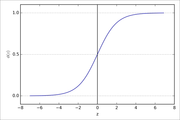
We can see that  approaches 1 if z goes towards infinity (
 ), since
  becomes very small for large values of z. Similarly, goes towards 0 for
  as the result of an increasingly large denominator. Thus, we conclude that this sigmoid function takes real number values as input and transforms them to values in the range [0, 1] with an intercept at
  .
.
To build some intuition for the logistic regression model, we can relate it to our previous Adaline implementation in Chapter 2, Training Machine Learning Algorithms for Classification. In Adaline, we used the identity function  as the activation function. In logistic regression, this activation function simply becomes the sigmoid function that we defined earlier, which is illustrated in the following figure:
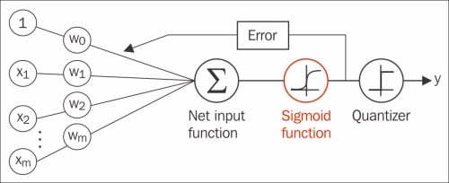
The output of the sigmoid function is then interpreted as the probability of particular sample belonging to class 1  , given its features x parameterized by the weights w. For example, if we compute
  for a particular flower sample, it means that the chance that this sample is an Iris-Versicolor flower is 80 percent. Similarly, the probability that this flower is an Iris-Setosa flower can be calculated as
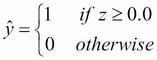
  or 20 percent. The predicted probability can then simply be converted into a binary outcome via a quantizer (unit step function):
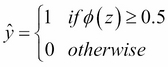
If we look at the preceding sigmoid plot, this is equivalent to the following:
In fact, there are many applications where we are not only interested in the predicted class labels, but where estimating the class-membership probability is particularly useful. Logistic regression is used in weather forecasting, for example, to not only predict if it will rain on a particular day but also to report the chance of rain. Similarly, logistic regression can be used to predict the chance that a patient has a particular disease given certain symptoms, which is why logistic regression enjoys wide popularity in the field of medicine.
You learned how we could use the logistic regression model to predict probabilities and class labels. Now let's briefly talk about the parameters of the model, for example, weights w. In the previous chapter, we defined the sum-squared-error cost function:
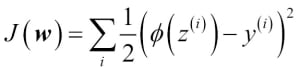
We minimized this in order to learn the weights w for our Adaline classification model. To explain how we can derive the cost function for logistic regression, let's first define the likelihood L that we want to maximize when we build a logistic regression model, assuming that the individual samples in our dataset are independent of one another. The formula is as follows:
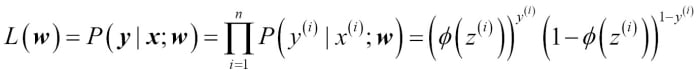
In practice, it is easier to maximize the (natural) log of this equation, which is called the log-likelihood function:
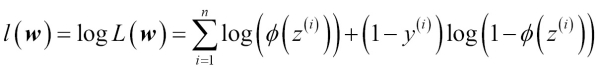
Firstly, applying the log function reduces the potential for numerical underflow, which can occur if the likelihoods are very small. Secondly, we can convert the product of factors into a summation of factors, which makes it easier to obtain the derivative of this function via the addition trick, as you may remember from calculus.
Now we could use an optimization algorithm such as gradient ascent to maximize this log-likelihood function. Alternatively, let's rewrite the log-likelihood as a cost function  that can be minimized using gradient descent as in Chapter 2, Training Machine Learning Algorithms for Classification:
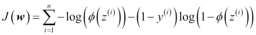
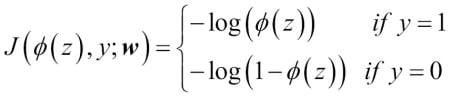
To get a better grasp on this cost function, let's take a look at the cost that we calculate for one single-sample instance:

Looking at the preceding equation, we can see that the first term becomes zero if  , and the second term becomes zero if , respectively:
The following plot illustrates the cost for the classification of a single-sample instance for different values of :
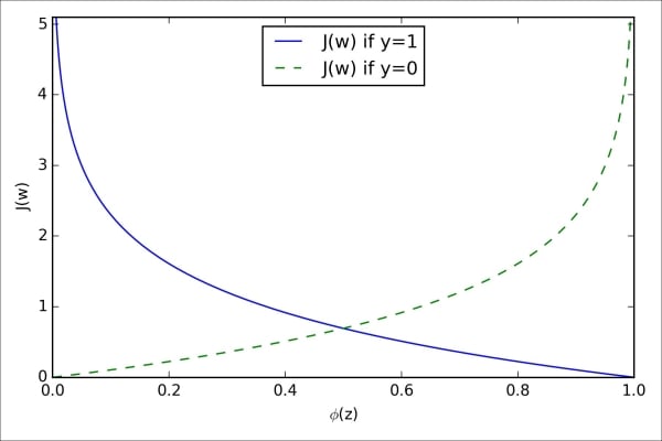
We can see that the cost approaches 0 (plain blue line) if we correctly predict that a sample belongs to class 1. Similarly, we can see on the y axis that the cost also approaches 0 if we correctly predict (dashed line). However, if the prediction is wrong, the cost goes towards infinity. The moral is that we penalize wrong predictions with an increasingly larger cost.
If we were to implement logistic regression ourselves, we could simply substitute the cost function in our Adaline implementation from Chapter 2, Training Machine Learning Algorithms for Classification, by the new cost function:
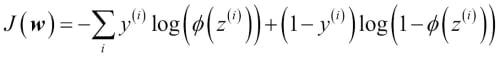
This would compute the cost of classifying all training samples per epoch and we would end up with a working logistic regression model. However, since scikit-learn implements a highly optimized version of logistic regression that also supports multiclass settings off-the-shelf, we will skip the implementation and use the sklearn.linear_model.LogisticRegression class as well as the familiar fit method to train the model on the standardized flower training dataset:
>>> from sklearn.linear_model import LogisticRegression
>>> lr = LogisticRegression(C=1000.0, random_state=0)
>>> lr.fit(X_train_std, y_train)
>>> plot_decision_regions(X_combined_std,
... y_combined, classifier=lr,
... test_idx=range(105,150))
>>> plt.xlabel('petal length [standardized]')
>>> plt.ylabel('petal width [standardized]')
>>> plt.legend(loc='upper left')
>>> plt.show()After fitting the model on the training data, we plotted the decision regions, training samples and test samples, as shown here:
Looking at the preceding code that we used to train the LogisticRegression model, you might now be wondering, "What is this mysterious parameter C?" We will get to this in a second, but let's briefly go over the concept of overfitting and regularization in the next subsection first.
Furthermore, we can predict the class-membership probability of the samples via the predict_proba method. For example, we can predict the probabilities of the first Iris-Setosa sample:
>>> lr.predict_proba(X_test_std[0,:])
This returns the following array:
array([[ 0.000, 0.063, 0.937]])
The preceding array tells us that the model predicts a chance of 93.7 percent that the sample belongs to the Iris-Virginica class, and a 6.3 percent chance that the sample is a Iris-Versicolor flower.
We can show that the weight update in logistic regression via gradient descent is indeed equal to the equation that we used in Adaline in Chapter 2, Training Machine Learning Algorithms for Classification. Let's start by calculating the partial derivative of the log-likelihood function with respect to the jth weight:
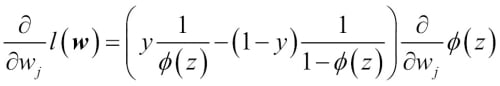
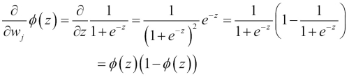
Before we continue, let's calculate the partial derivative of the sigmoid function first:
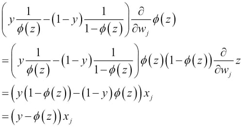
Now we can resubstitute  =
=  in our first equation to obtain the following:
Remember that the goal is to find the weights that maximize the log-likelihood so that we would perform the update for each weight as follows:
Since we update all weights simultaneously, we can write the general update rule as follows:
We define  as follows:
Since maximizing the log-likelihood is equal to minimizing the cost function that we defined earlier, we can write the gradient descent update rule as follows:
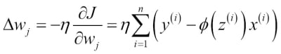
This is equal to the gradient descent rule in Adaline in Chapter 2, Training Machine Learning Algorithms for Classification.
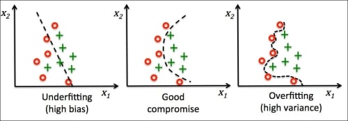
Overfitting is a common problem in machine learning, where a model performs well on training data but does not generalize well to unseen data (test data). If a model suffers from overfitting, we also say that the model has a high variance, which can be caused by having too many parameters that lead to a model that is too complex given the underlying data. Similarly, our model can also suffer from underfitting (high bias), which means that our model is not complex enough to capture the pattern in the training data well and therefore also suffers from low performance on unseen data.
Although we have only encountered linear models for classification so far, the problem of overfitting and underfitting can be best illustrated by using a more complex, nonlinear decision boundary as shown in the following figure:
Note
Variance measures the consistency (or variability) of the model prediction for a particular sample instance if we would retrain the model multiple times, for example, on different subsets of the training dataset. We can say that the model is sensitive to the randomness in the training data. In contrast, bias measures how far off the predictions are from the correct values in general if we rebuild the model multiple times on different training datasets; bias is the measure of the systematic error that is not due to randomness.
One way of finding a good bias-variance tradeoff is to tune the complexity of the model via regularization. Regularization is a very useful method to handle collinearity (high correlation among features), filter out noise from data, and eventually prevent overfitting. The concept behind regularization is to introduce additional information (bias) to penalize extreme parameter weights. The most common form of regularization is the so-called L2 regularization (sometimes also called L2 shrinkage or weight decay), which can be written as follows:
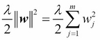
Here,  is the so-called regularization parameter.
In order to apply regularization, we just need to add the regularization term to the cost function that we defined for logistic regression to shrink the weights:
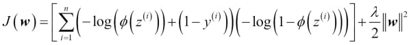
Via the regularization parameter , we can then control how well we fit the training data while keeping the weights small. By increasing the value of , we increase the regularization strength.
The parameter C that is implemented for the LogisticRegression class in scikit-learn comes from a convention in support vector machines, which will be the topic of the next section. C is directly related to the regularization parameter , which is its inverse:

So we can rewrite the regularized cost function of logistic regression as follows:

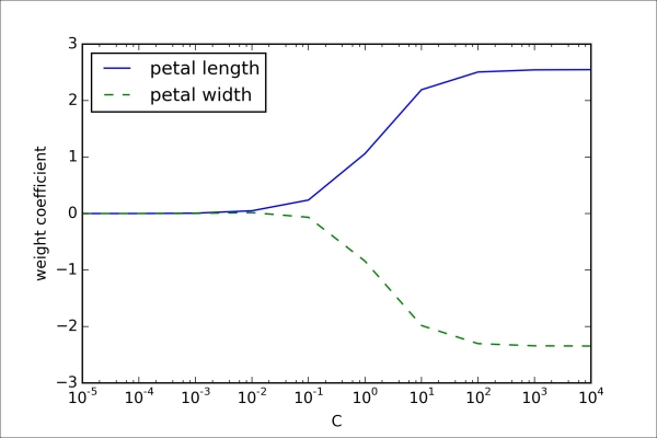
Consequently, decreasing the value of the inverse regularization parameter C means that we are increasing the regularization strength, which we can visualize by plotting the L2 regularization path for the two weight coefficients:
>>> weights, params = [], []
>>> for c in np.arange(-5, 5):
... lr = LogisticRegression(C=10**c, random_state=0)
... lr.fit(X_train_std, y_train)
... weights.append(lr.coef_[1])
... params.append(10**c)
>>> weights = np.array(weights)
>>> plt.plot(params, weights[:, 0],
... label='petal length')
>>> plt.plot(params, weights[:, 1], linestyle='--',
... label='petal width')
>>> plt.ylabel('weight coefficient')
>>> plt.xlabel('C')
>>> plt.legend(loc='upper left')
>>> plt.xscale('log')
>>> plt.show()By executing the preceding code, we fitted ten logistic regression models with different values for the inverse-regularization parameter C. For the purposes of illustration, we only collected the weight coefficients of the class 2 vs. all classifier. Remember that we are using the OvR technique for multiclass classification.
As we can see in the resulting plot, the weight coefficients shrink if we decrease the parameter C, that is, if we increase the regularization strength:
Note
Since an in-depth coverage of the individual classification algorithms exceeds the scope of this book, I warmly recommend Dr. Scott Menard's Logistic Regression: From Introductory to Advanced Concepts and Applications, Sage Publications, to readers who want to learn more about logistic regression.
Logistic regression intuition and conditional probabilities
Logistic regression is a classification model that is very easy to implement but performs very well on linearly separable classes. It is one of the most widely used algorithms for classification in industry. Similar to the perceptron and Adaline, the logistic regression model in this chapter is also a linear model for binary classification that can be extended to multiclass classification via the OvR technique.
To explain the idea behind logistic regression as a probabilistic model, let's first introduce the
odds ratio, which is the odds in favor of a particular event. The odds ratio can be written as , where stands for the probability of the positive event. The term positive event does not necessarily mean good, but refers to the event that we want to predict, for example, the probability that a patient has a certain disease; we can think of the positive event as class label . We can then further define the
logit function, which is simply the logarithm of the odds ratio (log-odds):
The logit function takes input values in the range 0 to 1 and transforms them to values over the entire real number range, which we can use to express a linear relationship between feature values and the log-odds:
Here, is the conditional probability that a particular sample belongs to class 1 given its features x.
Now what we are actually interested in is predicting the probability that a certain sample belongs to a particular class, which is the inverse form of the logit function. It is also called the logistic function, sometimes simply abbreviated as sigmoid function due to its characteristic S-shape.
Here, z is the net input, that is, the linear combination of weights and sample features and can be calculated as .
Now let's simply plot the sigmoid function for some values in the range -7 to 7 to see what it looks like:
>>> import matplotlib.pyplot as plt
>>> import numpy as np
>>> def sigmoid(z):
... return 1.0 / (1.0 + np.exp(-z))
>>> z = np.arange(-7, 7, 0.1)
>>> phi_z = sigmoid(z)
>>> plt.plot(z, phi_z)
>>> plt.axvline(0.0, color='k')
>>> plt.axhspan(0.0, 1.0, facecolor='1.0', alpha=1.0, ls='dotted')
>>> plt.axhline(y=0.5, ls='dotted', color='k')
>>> plt.yticks([0.0, 0.5, 1.0])
>>> plt.ylim(-0.1, 1.1)
>>> plt.xlabel('z')
>>> plt.ylabel('$\phi (z)$')
>>> plt.show() As a result of executing the previous code example, we should now see the S-shaped (sigmoidal) curve:
We can see that approaches 1 if z goes towards infinity (), since becomes very small for large values of z. Similarly, goes towards 0 for as the result of an increasingly large denominator. Thus, we conclude that this sigmoid function takes real number values as input and transforms them to values in the range [0, 1] with an intercept at .
To build some intuition for the logistic regression model, we can relate it to our previous Adaline implementation in Chapter 2, Training Machine Learning Algorithms for Classification. In Adaline, we used the identity function as the activation function. In logistic regression, this activation function simply becomes the sigmoid function that we defined earlier, which is illustrated in the following figure:
The output of the sigmoid function is then interpreted as the probability of particular sample belonging to class 1 , given its features x parameterized by the weights w. For example, if we compute for a particular flower sample, it means that the chance that this sample is an Iris-Versicolor flower is 80 percent. Similarly, the probability that this flower is an Iris-Setosa flower can be calculated as or 20 percent. The predicted probability can then simply be converted into a binary outcome via a quantizer (unit step function):
If we look at the preceding sigmoid plot, this is equivalent to the following:
In fact, there are many applications where we are not only interested in the predicted class labels, but where estimating the class-membership probability is particularly useful. Logistic regression is used in weather forecasting, for example, to not only predict if it will rain on a particular day but also to report the chance of rain. Similarly, logistic regression can be used to predict the chance that a patient has a particular disease given certain symptoms, which is why logistic regression enjoys wide popularity in the field of medicine.
You learned how we could use the logistic regression model to predict probabilities and class labels. Now let's briefly talk about the parameters of the model, for example, weights w. In the previous chapter, we defined the sum-squared-error cost function:
We minimized this in order to learn the weights w for our Adaline classification model. To explain how we can derive the cost function for logistic regression, let's first define the likelihood L that we want to maximize when we build a logistic regression model, assuming that the individual samples in our dataset are independent of one another. The formula is as follows:
In practice, it is easier to maximize the (natural) log of this equation, which is called the log-likelihood function:
Firstly, applying the log function reduces the potential for numerical underflow, which can occur if the likelihoods are very small. Secondly, we can convert the product of factors into a summation of factors, which makes it easier to obtain the derivative of this function via the addition trick, as you may remember from calculus.
Now we could use an optimization algorithm such as gradient ascent to maximize this log-likelihood function. Alternatively, let's rewrite the log-likelihood as a cost function that can be minimized using gradient descent as in Chapter 2, Training Machine Learning Algorithms for Classification:
To get a better grasp on this cost function, let's take a look at the cost that we calculate for one single-sample instance:
Looking at the preceding equation, we can see that the first term becomes zero if , and the second term becomes zero if , respectively:
The following plot illustrates the cost for the classification of a single-sample instance for different values of :
We can see that the cost approaches 0 (plain blue line) if we correctly predict that a sample belongs to class 1. Similarly, we can see on the y axis that the cost also approaches 0 if we correctly predict (dashed line). However, if the prediction is wrong, the cost goes towards infinity. The moral is that we penalize wrong predictions with an increasingly larger cost.
If we were to implement logistic regression ourselves, we could simply substitute the cost function in our Adaline implementation from Chapter 2, Training Machine Learning Algorithms for Classification, by the new cost function:
This would compute the cost of classifying all training samples per epoch and we would end up with a working logistic regression model. However, since scikit-learn implements a highly optimized version of logistic regression that also supports multiclass settings off-the-shelf, we will skip the implementation and use the sklearn.linear_model.LogisticRegression class as well as the familiar fit method to train the model on the standardized flower training dataset:
>>> from sklearn.linear_model import LogisticRegression
>>> lr = LogisticRegression(C=1000.0, random_state=0)
>>> lr.fit(X_train_std, y_train)
>>> plot_decision_regions(X_combined_std,
... y_combined, classifier=lr,
... test_idx=range(105,150))
>>> plt.xlabel('petal length [standardized]')
>>> plt.ylabel('petal width [standardized]')
>>> plt.legend(loc='upper left')
>>> plt.show()After fitting the model on the training data, we plotted the decision regions, training samples and test samples, as shown here:
Looking at the preceding code that we used to train the LogisticRegression model, you might now be wondering, "What is this mysterious parameter C?" We will get to this in a second, but let's briefly go over the concept of overfitting and regularization in the next subsection first.
Furthermore, we can predict the class-membership probability of the samples via the predict_proba method. For example, we can predict the probabilities of the first Iris-Setosa sample:
>>> lr.predict_proba(X_test_std[0,:])
This returns the following array:
array([[ 0.000, 0.063, 0.937]])
The preceding array tells us that the model predicts a chance of 93.7 percent that the sample belongs to the Iris-Virginica class, and a 6.3 percent chance that the sample is a Iris-Versicolor flower.
We can show that the weight update in logistic regression via gradient descent is indeed equal to the equation that we used in Adaline in Chapter 2, Training Machine Learning Algorithms for Classification. Let's start by calculating the partial derivative of the log-likelihood function with respect to the jth weight:
Before we continue, let's calculate the partial derivative of the sigmoid function first:
Now we can resubstitute = in our first equation to obtain the following:
Remember that the goal is to find the weights that maximize the log-likelihood so that we would perform the update for each weight as follows:
Since we update all weights simultaneously, we can write the general update rule as follows:
We define as follows:
Since maximizing the log-likelihood is equal to minimizing the cost function that we defined earlier, we can write the gradient descent update rule as follows:
This is equal to the gradient descent rule in Adaline in Chapter 2, Training Machine Learning Algorithms for Classification.
Overfitting is a common problem in machine learning, where a model performs well on training data but does not generalize well to unseen data (test data). If a model suffers from overfitting, we also say that the model has a high variance, which can be caused by having too many parameters that lead to a model that is too complex given the underlying data. Similarly, our model can also suffer from underfitting (high bias), which means that our model is not complex enough to capture the pattern in the training data well and therefore also suffers from low performance on unseen data.
Although we have only encountered linear models for classification so far, the problem of overfitting and underfitting can be best illustrated by using a more complex, nonlinear decision boundary as shown in the following figure:
Note
Variance measures the consistency (or variability) of the model prediction for a particular sample instance if we would retrain the model multiple times, for example, on different subsets of the training dataset. We can say that the model is sensitive to the randomness in the training data. In contrast, bias measures how far off the predictions are from the correct values in general if we rebuild the model multiple times on different training datasets; bias is the measure of the systematic error that is not due to randomness.
One way of finding a good bias-variance tradeoff is to tune the complexity of the model via regularization. Regularization is a very useful method to handle collinearity (high correlation among features), filter out noise from data, and eventually prevent overfitting. The concept behind regularization is to introduce additional information (bias) to penalize extreme parameter weights. The most common form of regularization is the so-called L2 regularization (sometimes also called L2 shrinkage or weight decay), which can be written as follows:
Here, is the so-called regularization parameter.
In order to apply regularization, we just need to add the regularization term to the cost function that we defined for logistic regression to shrink the weights:
Via the regularization parameter , we can then control how well we fit the training data while keeping the weights small. By increasing the value of , we increase the regularization strength.
The parameter C that is implemented for the LogisticRegression class in scikit-learn comes from a convention in support vector machines, which will be the topic of the next section. C is directly related to the regularization parameter , which is its inverse:
So we can rewrite the regularized cost function of logistic regression as follows:
Consequently, decreasing the value of the inverse regularization parameter C means that we are increasing the regularization strength, which we can visualize by plotting the L2 regularization path for the two weight coefficients:
>>> weights, params = [], []
>>> for c in np.arange(-5, 5):
... lr = LogisticRegression(C=10**c, random_state=0)
... lr.fit(X_train_std, y_train)
... weights.append(lr.coef_[1])
... params.append(10**c)
>>> weights = np.array(weights)
>>> plt.plot(params, weights[:, 0],
... label='petal length')
>>> plt.plot(params, weights[:, 1], linestyle='--',
... label='petal width')
>>> plt.ylabel('weight coefficient')
>>> plt.xlabel('C')
>>> plt.legend(loc='upper left')
>>> plt.xscale('log')
>>> plt.show()By executing the preceding code, we fitted ten logistic regression models with different values for the inverse-regularization parameter C. For the purposes of illustration, we only collected the weight coefficients of the class 2 vs. all classifier. Remember that we are using the OvR technique for multiclass classification.
As we can see in the resulting plot, the weight coefficients shrink if we decrease the parameter C, that is, if we increase the regularization strength:
Note
Since an in-depth coverage of the individual classification algorithms exceeds the scope of this book, I warmly recommend Dr. Scott Menard's Logistic Regression: From Introductory to Advanced Concepts and Applications, Sage Publications, to readers who want to learn more about logistic regression.
Learning the weights of the logistic cost function
You learned how we could use the logistic regression model to predict probabilities and class labels. Now let's briefly talk about the parameters of the model, for example, weights w. In the previous chapter, we defined the sum-squared-error cost function:
We minimized this in order to learn the weights w for our Adaline classification model. To explain how we can derive the cost function for logistic regression, let's first define the likelihood L that we want to maximize when we build a logistic regression model, assuming that the individual samples in our dataset are independent of one another. The formula is as follows:
In practice, it is easier to maximize the (natural) log of this equation, which is called the log-likelihood function:
Firstly, applying the log function reduces the potential for numerical underflow, which can occur if the likelihoods are very small. Secondly, we can convert the product of factors into a summation of factors, which makes it easier to obtain the derivative of this function via the addition trick, as you may remember from calculus.
Now we could use an optimization algorithm such as gradient ascent to maximize this log-likelihood function. Alternatively, let's rewrite the log-likelihood as a cost function that can be minimized using gradient descent as in Chapter 2, Training Machine Learning Algorithms for Classification:
To get a better grasp on this cost function, let's take a look at the cost that we calculate for one single-sample instance:
Looking at the preceding equation, we can see that the first term becomes zero if , and the second term becomes zero if , respectively:
The following plot illustrates the cost for the classification of a single-sample instance for different values of :
We can see that the cost approaches 0 (plain blue line) if we correctly predict that a sample belongs to class 1. Similarly, we can see on the y axis that the cost also approaches 0 if we correctly predict (dashed line). However, if the prediction is wrong, the cost goes towards infinity. The moral is that we penalize wrong predictions with an increasingly larger cost.
If we were to implement logistic regression ourselves, we could simply substitute the cost function in our Adaline implementation from Chapter 2, Training Machine Learning Algorithms for Classification, by the new cost function:
This would compute the cost of classifying all training samples per epoch and we would end up with a working logistic regression model. However, since scikit-learn implements a highly optimized version of logistic regression that also supports multiclass settings off-the-shelf, we will skip the implementation and use the sklearn.linear_model.LogisticRegression class as well as the familiar fit method to train the model on the standardized flower training dataset:
>>> from sklearn.linear_model import LogisticRegression
>>> lr = LogisticRegression(C=1000.0, random_state=0)
>>> lr.fit(X_train_std, y_train)
>>> plot_decision_regions(X_combined_std,
... y_combined, classifier=lr,
... test_idx=range(105,150))
>>> plt.xlabel('petal length [standardized]')
>>> plt.ylabel('petal width [standardized]')
>>> plt.legend(loc='upper left')
>>> plt.show()After fitting the model on the training data, we plotted the decision regions, training samples and test samples, as shown here:
Looking at the preceding code that we used to train the LogisticRegression model, you might now be wondering, "What is this mysterious parameter C?" We will get to this in a second, but let's briefly go over the concept of overfitting and regularization in the next subsection first.
Furthermore, we can predict the class-membership probability of the samples via the predict_proba method. For example, we can predict the probabilities of the first Iris-Setosa sample:
>>> lr.predict_proba(X_test_std[0,:])
This returns the following array:
array([[ 0.000, 0.063, 0.937]])
The preceding array tells us that the model predicts a chance of 93.7 percent that the sample belongs to the Iris-Virginica class, and a 6.3 percent chance that the sample is a Iris-Versicolor flower.
We can show that the weight update in logistic regression via gradient descent is indeed equal to the equation that we used in Adaline in Chapter 2, Training Machine Learning Algorithms for Classification. Let's start by calculating the partial derivative of the log-likelihood function with respect to the jth weight:
Before we continue, let's calculate the partial derivative of the sigmoid function first:
Now we can resubstitute = in our first equation to obtain the following:
Remember that the goal is to find the weights that maximize the log-likelihood so that we would perform the update for each weight as follows:
Since we update all weights simultaneously, we can write the general update rule as follows:
We define as follows:
Since maximizing the log-likelihood is equal to minimizing the cost function that we defined earlier, we can write the gradient descent update rule as follows:
This is equal to the gradient descent rule in Adaline in Chapter 2, Training Machine Learning Algorithms for Classification.
Overfitting is a common problem in machine learning, where a model performs well on training data but does not generalize well to unseen data (test data). If a model suffers from overfitting, we also say that the model has a high variance, which can be caused by having too many parameters that lead to a model that is too complex given the underlying data. Similarly, our model can also suffer from underfitting (high bias), which means that our model is not complex enough to capture the pattern in the training data well and therefore also suffers from low performance on unseen data.
Although we have only encountered linear models for classification so far, the problem of overfitting and underfitting can be best illustrated by using a more complex, nonlinear decision boundary as shown in the following figure:
Note
Variance measures the consistency (or variability) of the model prediction for a particular sample instance if we would retrain the model multiple times, for example, on different subsets of the training dataset. We can say that the model is sensitive to the randomness in the training data. In contrast, bias measures how far off the predictions are from the correct values in general if we rebuild the model multiple times on different training datasets; bias is the measure of the systematic error that is not due to randomness.
One way of finding a good bias-variance tradeoff is to tune the complexity of the model via regularization. Regularization is a very useful method to handle collinearity (high correlation among features), filter out noise from data, and eventually prevent overfitting. The concept behind regularization is to introduce additional information (bias) to penalize extreme parameter weights. The most common form of regularization is the so-called L2 regularization (sometimes also called L2 shrinkage or weight decay), which can be written as follows:
Here, is the so-called regularization parameter.
In order to apply regularization, we just need to add the regularization term to the cost function that we defined for logistic regression to shrink the weights:
Via the regularization parameter , we can then control how well we fit the training data while keeping the weights small. By increasing the value of , we increase the regularization strength.
The parameter C that is implemented for the LogisticRegression class in scikit-learn comes from a convention in support vector machines, which will be the topic of the next section. C is directly related to the regularization parameter , which is its inverse:
So we can rewrite the regularized cost function of logistic regression as follows:
Consequently, decreasing the value of the inverse regularization parameter C means that we are increasing the regularization strength, which we can visualize by plotting the L2 regularization path for the two weight coefficients:
>>> weights, params = [], []
>>> for c in np.arange(-5, 5):
... lr = LogisticRegression(C=10**c, random_state=0)
... lr.fit(X_train_std, y_train)
... weights.append(lr.coef_[1])
... params.append(10**c)
>>> weights = np.array(weights)
>>> plt.plot(params, weights[:, 0],
... label='petal length')
>>> plt.plot(params, weights[:, 1], linestyle='--',
... label='petal width')
>>> plt.ylabel('weight coefficient')
>>> plt.xlabel('C')
>>> plt.legend(loc='upper left')
>>> plt.xscale('log')
>>> plt.show()By executing the preceding code, we fitted ten logistic regression models with different values for the inverse-regularization parameter C. For the purposes of illustration, we only collected the weight coefficients of the class 2 vs. all classifier. Remember that we are using the OvR technique for multiclass classification.
As we can see in the resulting plot, the weight coefficients shrink if we decrease the parameter C, that is, if we increase the regularization strength:
Note
Since an in-depth coverage of the individual classification algorithms exceeds the scope of this book, I warmly recommend Dr. Scott Menard's Logistic Regression: From Introductory to Advanced Concepts and Applications, Sage Publications, to readers who want to learn more about logistic regression.
Training a logistic regression model with scikit-learn
If we were to implement logistic regression ourselves, we could simply substitute the cost function in our Adaline implementation from Chapter 2, Training Machine Learning Algorithms for Classification, by the new cost function:
This would compute the cost of classifying all training samples per epoch and we would end up with a working logistic regression model. However, since scikit-learn implements a highly optimized version of logistic regression that also supports multiclass settings off-the-shelf, we will skip the implementation and use the sklearn.linear_model.LogisticRegression class as well as the familiar fit method to train the model on the standardized flower training dataset:
>>> from sklearn.linear_model import LogisticRegression
>>> lr = LogisticRegression(C=1000.0, random_state=0)
>>> lr.fit(X_train_std, y_train)
>>> plot_decision_regions(X_combined_std,
... y_combined, classifier=lr,
... test_idx=range(105,150))
>>> plt.xlabel('petal length [standardized]')
>>> plt.ylabel('petal width [standardized]')
>>> plt.legend(loc='upper left')
>>> plt.show()After fitting the model on the training data, we plotted the decision regions, training samples and test samples, as shown here:
Looking at the preceding code that we used to train the LogisticRegression model, you might now be wondering, "What is this mysterious parameter C?" We will get to this in a second, but let's briefly go over the concept of overfitting and regularization in the next subsection first.
Furthermore, we can predict the class-membership probability of the samples via the predict_proba method. For example, we can predict the probabilities of the first Iris-Setosa sample:
>>> lr.predict_proba(X_test_std[0,:])
This returns the following array:
array([[ 0.000, 0.063, 0.937]])
The preceding array tells us that the model predicts a chance of 93.7 percent that the sample belongs to the Iris-Virginica class, and a 6.3 percent chance that the sample is a Iris-Versicolor flower.
We can show that the weight update in logistic regression via gradient descent is indeed equal to the equation that we used in Adaline in Chapter 2, Training Machine Learning Algorithms for Classification. Let's start by calculating the partial derivative of the log-likelihood function with respect to the jth weight:
Before we continue, let's calculate the partial derivative of the sigmoid function first:
Now we can resubstitute = in our first equation to obtain the following:
Remember that the goal is to find the weights that maximize the log-likelihood so that we would perform the update for each weight as follows:
Since we update all weights simultaneously, we can write the general update rule as follows:
We define as follows:
Since maximizing the log-likelihood is equal to minimizing the cost function that we defined earlier, we can write the gradient descent update rule as follows:
This is equal to the gradient descent rule in Adaline in Chapter 2, Training Machine Learning Algorithms for Classification.
Overfitting is a common problem in machine learning, where a model performs well on training data but does not generalize well to unseen data (test data). If a model suffers from overfitting, we also say that the model has a high variance, which can be caused by having too many parameters that lead to a model that is too complex given the underlying data. Similarly, our model can also suffer from underfitting (high bias), which means that our model is not complex enough to capture the pattern in the training data well and therefore also suffers from low performance on unseen data.
Although we have only encountered linear models for classification so far, the problem of overfitting and underfitting can be best illustrated by using a more complex, nonlinear decision boundary as shown in the following figure:
Note
Variance measures the consistency (or variability) of the model prediction for a particular sample instance if we would retrain the model multiple times, for example, on different subsets of the training dataset. We can say that the model is sensitive to the randomness in the training data. In contrast, bias measures how far off the predictions are from the correct values in general if we rebuild the model multiple times on different training datasets; bias is the measure of the systematic error that is not due to randomness.
One way of finding a good bias-variance tradeoff is to tune the complexity of the model via regularization. Regularization is a very useful method to handle collinearity (high correlation among features), filter out noise from data, and eventually prevent overfitting. The concept behind regularization is to introduce additional information (bias) to penalize extreme parameter weights. The most common form of regularization is the so-called L2 regularization (sometimes also called L2 shrinkage or weight decay), which can be written as follows:
Here, is the so-called regularization parameter.
In order to apply regularization, we just need to add the regularization term to the cost function that we defined for logistic regression to shrink the weights:
Via the regularization parameter , we can then control how well we fit the training data while keeping the weights small. By increasing the value of , we increase the regularization strength.
The parameter C that is implemented for the LogisticRegression class in scikit-learn comes from a convention in support vector machines, which will be the topic of the next section. C is directly related to the regularization parameter , which is its inverse:
So we can rewrite the regularized cost function of logistic regression as follows:
Consequently, decreasing the value of the inverse regularization parameter C means that we are increasing the regularization strength, which we can visualize by plotting the L2 regularization path for the two weight coefficients:
>>> weights, params = [], []
>>> for c in np.arange(-5, 5):
... lr = LogisticRegression(C=10**c, random_state=0)
... lr.fit(X_train_std, y_train)
... weights.append(lr.coef_[1])
... params.append(10**c)
>>> weights = np.array(weights)
>>> plt.plot(params, weights[:, 0],
... label='petal length')
>>> plt.plot(params, weights[:, 1], linestyle='--',
... label='petal width')
>>> plt.ylabel('weight coefficient')
>>> plt.xlabel('C')
>>> plt.legend(loc='upper left')
>>> plt.xscale('log')
>>> plt.show()By executing the preceding code, we fitted ten logistic regression models with different values for the inverse-regularization parameter C. For the purposes of illustration, we only collected the weight coefficients of the class 2 vs. all classifier. Remember that we are using the OvR technique for multiclass classification.
As we can see in the resulting plot, the weight coefficients shrink if we decrease the parameter C, that is, if we increase the regularization strength:
Note
Since an in-depth coverage of the individual classification algorithms exceeds the scope of this book, I warmly recommend Dr. Scott Menard's Logistic Regression: From Introductory to Advanced Concepts and Applications, Sage Publications, to readers who want to learn more about logistic regression.
Tackling overfitting via regularization
Overfitting is a common problem in machine learning, where a model performs well on training data but does not generalize well to unseen data (test data). If a model suffers from overfitting, we also say that the model has a high variance, which can be caused by having too many parameters that lead to a model that is too complex given the underlying data. Similarly, our model can also suffer from underfitting (high bias), which means that our model is not complex enough to capture the pattern in the training data well and therefore also suffers from low performance on unseen data.
Although we have only encountered linear models for classification so far, the problem of overfitting and underfitting can be best illustrated by using a more complex, nonlinear decision boundary as shown in the following figure:
Note
Variance measures the consistency (or variability) of the model prediction for a particular sample instance if we would retrain the model multiple times, for example, on different subsets of the training dataset. We can say that the model is sensitive to the randomness in the training data. In contrast, bias measures how far off the predictions are from the correct values in general if we rebuild the model multiple times on different training datasets; bias is the measure of the systematic error that is not due to randomness.
One way of finding a good bias-variance tradeoff is to tune the complexity of the model via regularization. Regularization is a very useful method to handle collinearity (high correlation among features), filter out noise from data, and eventually prevent overfitting. The concept behind regularization is to introduce additional information (bias) to penalize extreme parameter weights. The most common form of regularization is the so-called L2 regularization (sometimes also called L2 shrinkage or weight decay), which can be written as follows:
Here, is the so-called regularization parameter.
In order to apply regularization, we just need to add the regularization term to the cost function that we defined for logistic regression to shrink the weights:
Via the regularization parameter , we can then control how well we fit the training data while keeping the weights small. By increasing the value of , we increase the regularization strength.
The parameter C that is implemented for the LogisticRegression class in scikit-learn comes from a convention in support vector machines, which will be the topic of the next section. C is directly related to the regularization parameter , which is its inverse:
So we can rewrite the regularized cost function of logistic regression as follows:
Consequently, decreasing the value of the inverse regularization parameter C means that we are increasing the regularization strength, which we can visualize by plotting the L2 regularization path for the two weight coefficients:
>>> weights, params = [], []
>>> for c in np.arange(-5, 5):
... lr = LogisticRegression(C=10**c, random_state=0)
... lr.fit(X_train_std, y_train)
... weights.append(lr.coef_[1])
... params.append(10**c)
>>> weights = np.array(weights)
>>> plt.plot(params, weights[:, 0],
... label='petal length')
>>> plt.plot(params, weights[:, 1], linestyle='--',
... label='petal width')
>>> plt.ylabel('weight coefficient')
>>> plt.xlabel('C')
>>> plt.legend(loc='upper left')
>>> plt.xscale('log')
>>> plt.show()By executing the preceding code, we fitted ten logistic regression models with different values for the inverse-regularization parameter C. For the purposes of illustration, we only collected the weight coefficients of the class 2 vs. all classifier. Remember that we are using the OvR technique for multiclass classification.
As we can see in the resulting plot, the weight coefficients shrink if we decrease the parameter C, that is, if we increase the regularization strength:
Note
Since an in-depth coverage of the individual classification algorithms exceeds the scope of this book, I warmly recommend Dr. Scott Menard's Logistic Regression: From Introductory to Advanced Concepts and Applications, Sage Publications, to readers who want to learn more about logistic regression.
Another powerful and widely used learning algorithm is the support vector machine (SVM), which can be considered as an extension of the perceptron. Using the perceptron algorithm, we minimized misclassification errors. However, in SVMs, our optimization objective is to maximize the margin. The margin is defined as the distance between the separating hyperplane (decision boundary) and the training samples that are closest to this hyperplane, which are the so-called support vectors. This is illustrated in the following figure:
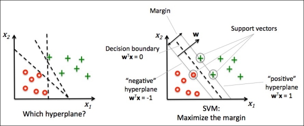
The rationale behind having decision boundaries with large margins is that they tend to have a lower generalization error whereas models with small margins are more prone to overfitting. To get an intuition for the margin maximization, let's take a closer look at those positive and negative hyperplanes that are parallel to the decision boundary, which can be expressed as follows:
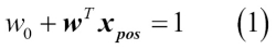
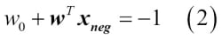
If we subtract those two linear equations (1) and (2) from each other, we get:
We can normalize this by the length of the vector w, which is defined as follows:
So we arrive at the following equation:
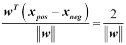
The left side of the preceding equation can then be interpreted as the distance between the positive and negative hyperplane, which is the so-called margin that we want to maximize.
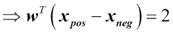
Now the objective function of the SVM becomes the maximization of this margin by maximizing  under the constraint that the samples are classified correctly, which can be written as follows:
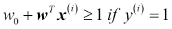
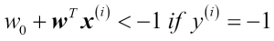
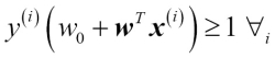
These two equations basically say that all negative samples should fall on one side of the negative hyperplane, whereas all the positive samples should fall behind the positive hyperplane. This can also be written more compactly as follows:
In practice, though, it is easier to minimize the reciprocal term  , which can be solved by quadratic programming. However, a detailed discussion about quadratic programming is beyond the scope of this book, but if you are interested, you can learn more about Support Vector Machines (SVM) in Vladimir Vapnik's The Nature of Statistical Learning Theory, Springer Science & Business Media, or Chris J.C. Burges' excellent explanation in A Tutorial on Support Vector Machines for Pattern Recognition (Data mining and knowledge discovery, 2(2):121–167, 1998).
Although we don't want to dive much deeper into the more involved mathematical concepts behind the margin classification, let's briefly mention the slack variable  . It was introduced by Vladimir Vapnik in 1995 and led to the so-called soft-margin classification. The motivation for introducing the slack variable was that the linear constraints need to be relaxed for nonlinearly separable data to allow convergence of the optimization in the presence of misclassifications under the appropriate cost penalization.
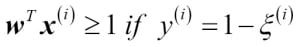
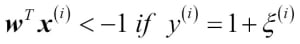
The positive-values slack variable is simply added to the linear constraints:
So the new objective to be minimized (subject to the preceding constraints) becomes:
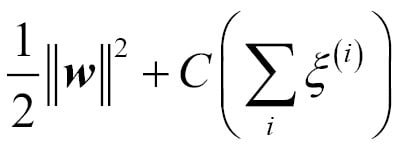
Using the variable C, we can then control the penalty for misclassification. Large values of C correspond to large error penalties whereas we are less strict about misclassification errors if we choose smaller values for C. We can then we use the parameter C to control the width of the margin and therefore tune the bias-variance trade-off as illustrated in the following figure:
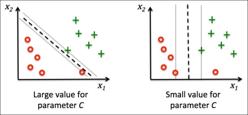
This concept is related to regularization, which we discussed previously in the context of regularized regression where increasing the value of C increases the bias and lowers the variance of the model.
Now that we learned the basic concepts behind the linear SVM, let's train a SVM model to classify the different flowers in our Iris dataset:
>>> from sklearn.svm import SVC
>>> svm = SVC(kernel='linear', C=1.0, random_state=0)
>>> svm.fit(X_train_std, y_train)
>>> plot_decision_regions(X_combined_std,
... y_combined, classifier=svm,
... test_idx=range(105,150))
>>> plt.xlabel('petal length [standardized]')
>>> plt.ylabel('petal width [standardized]')
>>> plt.legend(loc='upper left')
>>> plt.show()The decision regions of the SVM visualized after executing the preceding code example are shown in the following plot:
Note
Logistic regression versus SVM
In practical classification tasks, linear logistic regression and linear SVMs often yield very similar results. Logistic regression tries to maximize the conditional likelihoods of the training data, which makes it more prone to outliers than SVMs. The SVMs mostly care about the points that are closest to the decision boundary (support vectors). On the other hand, logistic regression has the advantage that it is a simpler model that can be implemented more easily. Furthermore, logistic regression models can be easily updated, which is attractive when working with streaming data.
The
Perceptron and LogisticRegression classes that we used in the previous sections via scikit-learn make use of the LIBLINEAR library, which is a highly optimized C/C++ library developed at the National Taiwan University (http://www.csie.ntu.edu.tw/~cjlin/liblinear/). Similarly, the SVC class that we used to train an SVM makes use of LIBSVM, which is an equivalent C/C++ library specialized for SVMs (http://www.csie.ntu.edu.tw/~cjlin/libsvm/).
The advantage of using LIBLINEAR and LIBSVM over native Python implementations is that they allow an extremely quick training of large amounts of linear classifiers. However, sometimes our datasets are too large to fit into computer memory. Thus, scikit-learn also offers alternative implementations via the SGDClassifier class, which also supports online learning via the partial_fit method. The concept behind the SGDClassifier class is similar to the stochastic gradient algorithm that we implemented in Chapter 2, Training Machine Learning Algorithms for Classification, for Adaline. We could initialize the stochastic gradient descent version of the perceptron, logistic regression, and support vector machine with default parameters as follows:
>>> from sklearn.linear_model import SGDClassifier >>> ppn = SGDClassifier(loss='perceptron') >>> lr = SGDClassifier(loss='log') >>> svm = SGDClassifier(loss='hinge')
Maximum margin intuition
The rationale behind having decision boundaries with large margins is that they tend to have a lower generalization error whereas models with small margins are more prone to overfitting. To get an intuition for the margin maximization, let's take a closer look at those positive and negative hyperplanes that are parallel to the decision boundary, which can be expressed as follows:
If we subtract those two linear equations (1) and (2) from each other, we get:
We can normalize this by the length of the vector w, which is defined as follows:
So we arrive at the following equation:
The left side of the preceding equation can then be interpreted as the distance between the positive and negative hyperplane, which is the so-called margin that we want to maximize.
Now the objective function of the SVM becomes the maximization of this margin by maximizing under the constraint that the samples are classified correctly, which can be written as follows:
These two equations basically say that all negative samples should fall on one side of the negative hyperplane, whereas all the positive samples should fall behind the positive hyperplane. This can also be written more compactly as follows:
In practice, though, it is easier to minimize the reciprocal term , which can be solved by quadratic programming. However, a detailed discussion about quadratic programming is beyond the scope of this book, but if you are interested, you can learn more about Support Vector Machines (SVM) in Vladimir Vapnik's The Nature of Statistical Learning Theory, Springer Science & Business Media, or Chris J.C. Burges' excellent explanation in A Tutorial on Support Vector Machines for Pattern Recognition (Data mining and knowledge discovery, 2(2):121–167, 1998).
Although we don't want to dive much deeper into the more involved mathematical concepts behind the margin classification, let's briefly mention the slack variable . It was introduced by Vladimir Vapnik in 1995 and led to the so-called soft-margin classification. The motivation for introducing the slack variable was that the linear constraints need to be relaxed for nonlinearly separable data to allow convergence of the optimization in the presence of misclassifications under the appropriate cost penalization.
The positive-values slack variable is simply added to the linear constraints:
So the new objective to be minimized (subject to the preceding constraints) becomes:
Using the variable C, we can then control the penalty for misclassification. Large values of C correspond to large error penalties whereas we are less strict about misclassification errors if we choose smaller values for C. We can then we use the parameter C to control the width of the margin and therefore tune the bias-variance trade-off as illustrated in the following figure:
This concept is related to regularization, which we discussed previously in the context of regularized regression where increasing the value of C increases the bias and lowers the variance of the model.
Now that we learned the basic concepts behind the linear SVM, let's train a SVM model to classify the different flowers in our Iris dataset:
>>> from sklearn.svm import SVC
>>> svm = SVC(kernel='linear', C=1.0, random_state=0)
>>> svm.fit(X_train_std, y_train)
>>> plot_decision_regions(X_combined_std,
... y_combined, classifier=svm,
... test_idx=range(105,150))
>>> plt.xlabel('petal length [standardized]')
>>> plt.ylabel('petal width [standardized]')
>>> plt.legend(loc='upper left')
>>> plt.show()The decision regions of the SVM visualized after executing the preceding code example are shown in the following plot:
Note
Logistic regression versus SVM
In practical classification tasks, linear logistic regression and linear SVMs often yield very similar results. Logistic regression tries to maximize the conditional likelihoods of the training data, which makes it more prone to outliers than SVMs. The SVMs mostly care about the points that are closest to the decision boundary (support vectors). On the other hand, logistic regression has the advantage that it is a simpler model that can be implemented more easily. Furthermore, logistic regression models can be easily updated, which is attractive when working with streaming data.
The
Perceptron and LogisticRegression classes that we used in the previous sections via scikit-learn make use of the LIBLINEAR library, which is a highly optimized C/C++ library developed at the National Taiwan University (http://www.csie.ntu.edu.tw/~cjlin/liblinear/). Similarly, the SVC class that we used to train an SVM makes use of LIBSVM, which is an equivalent C/C++ library specialized for SVMs (http://www.csie.ntu.edu.tw/~cjlin/libsvm/).
The advantage of using LIBLINEAR and LIBSVM over native Python implementations is that they allow an extremely quick training of large amounts of linear classifiers. However, sometimes our datasets are too large to fit into computer memory. Thus, scikit-learn also offers alternative implementations via the SGDClassifier class, which also supports online learning via the partial_fit method. The concept behind the SGDClassifier class is similar to the stochastic gradient algorithm that we implemented in Chapter 2, Training Machine Learning Algorithms for Classification, for Adaline. We could initialize the stochastic gradient descent version of the perceptron, logistic regression, and support vector machine with default parameters as follows:
>>> from sklearn.linear_model import SGDClassifier >>> ppn = SGDClassifier(loss='perceptron') >>> lr = SGDClassifier(loss='log') >>> svm = SGDClassifier(loss='hinge')
Dealing with the nonlinearly separable case using slack variables
Although we don't want to dive much deeper into the more involved mathematical concepts behind the margin classification, let's briefly mention the slack variable . It was introduced by Vladimir Vapnik in 1995 and led to the so-called soft-margin classification. The motivation for introducing the slack variable was that the linear constraints need to be relaxed for nonlinearly separable data to allow convergence of the optimization in the presence of misclassifications under the appropriate cost penalization.
The positive-values slack variable is simply added to the linear constraints:
So the new objective to be minimized (subject to the preceding constraints) becomes:
Using the variable C, we can then control the penalty for misclassification. Large values of C correspond to large error penalties whereas we are less strict about misclassification errors if we choose smaller values for C. We can then we use the parameter C to control the width of the margin and therefore tune the bias-variance trade-off as illustrated in the following figure:
This concept is related to regularization, which we discussed previously in the context of regularized regression where increasing the value of C increases the bias and lowers the variance of the model.
Now that we learned the basic concepts behind the linear SVM, let's train a SVM model to classify the different flowers in our Iris dataset:
>>> from sklearn.svm import SVC
>>> svm = SVC(kernel='linear', C=1.0, random_state=0)
>>> svm.fit(X_train_std, y_train)
>>> plot_decision_regions(X_combined_std,
... y_combined, classifier=svm,
... test_idx=range(105,150))
>>> plt.xlabel('petal length [standardized]')
>>> plt.ylabel('petal width [standardized]')
>>> plt.legend(loc='upper left')
>>> plt.show()The decision regions of the SVM visualized after executing the preceding code example are shown in the following plot:
Note
Logistic regression versus SVM
In practical classification tasks, linear logistic regression and linear SVMs often yield very similar results. Logistic regression tries to maximize the conditional likelihoods of the training data, which makes it more prone to outliers than SVMs. The SVMs mostly care about the points that are closest to the decision boundary (support vectors). On the other hand, logistic regression has the advantage that it is a simpler model that can be implemented more easily. Furthermore, logistic regression models can be easily updated, which is attractive when working with streaming data.
The
Perceptron and LogisticRegression classes that we used in the previous sections via scikit-learn make use of the LIBLINEAR library, which is a highly optimized C/C++ library developed at the National Taiwan University (http://www.csie.ntu.edu.tw/~cjlin/liblinear/). Similarly, the SVC class that we used to train an SVM makes use of LIBSVM, which is an equivalent C/C++ library specialized for SVMs (http://www.csie.ntu.edu.tw/~cjlin/libsvm/).
The advantage of using LIBLINEAR and LIBSVM over native Python implementations is that they allow an extremely quick training of large amounts of linear classifiers. However, sometimes our datasets are too large to fit into computer memory. Thus, scikit-learn also offers alternative implementations via the SGDClassifier class, which also supports online learning via the partial_fit method. The concept behind the SGDClassifier class is similar to the stochastic gradient algorithm that we implemented in Chapter 2, Training Machine Learning Algorithms for Classification, for Adaline. We could initialize the stochastic gradient descent version of the perceptron, logistic regression, and support vector machine with default parameters as follows:
>>> from sklearn.linear_model import SGDClassifier >>> ppn = SGDClassifier(loss='perceptron') >>> lr = SGDClassifier(loss='log') >>> svm = SGDClassifier(loss='hinge')
Alternative implementations in scikit-learn
The
Perceptron and LogisticRegression classes that we used in the previous sections via scikit-learn make use of the LIBLINEAR library, which is a highly optimized C/C++ library developed at the National Taiwan University (http://www.csie.ntu.edu.tw/~cjlin/liblinear/). Similarly, the SVC class that we used to train an SVM makes use of LIBSVM, which is an equivalent C/C++ library specialized for SVMs (http://www.csie.ntu.edu.tw/~cjlin/libsvm/).
The advantage of using LIBLINEAR and LIBSVM over native Python implementations is that they allow an extremely quick training of large amounts of linear classifiers. However, sometimes our datasets are too large to fit into computer memory. Thus, scikit-learn also offers alternative implementations via the SGDClassifier class, which also supports online learning via the partial_fit method. The concept behind the SGDClassifier class is similar to the stochastic gradient algorithm that we implemented in Chapter 2, Training Machine Learning Algorithms for Classification, for Adaline. We could initialize the stochastic gradient descent version of the perceptron, logistic regression, and support vector machine with default parameters as follows:
>>> from sklearn.linear_model import SGDClassifier >>> ppn = SGDClassifier(loss='perceptron') >>> lr = SGDClassifier(loss='log') >>> svm = SGDClassifier(loss='hinge')
Another reason why SVMs enjoy high popularity among machine learning practitioners is that they can be easily kernelized to solve nonlinear classification problems. Before we discuss the main concept behind kernel SVM, let's first define and create a sample dataset to see how such a nonlinear classification problem may look.
Using the following code, we will create a simple dataset that has the form of an XOR gate using the logical_xor function from NumPy, where 100 samples will be assigned the class label 1 and 100 samples will be assigned the class label -1, respectively:
>>> np.random.seed(0) >>> X_xor = np.random.randn(200, 2) >>> y_xor = np.logical_xor(X_xor[:, 0] > 0, X_xor[:, 1] > 0) >>> y_xor = np.where(y_xor, 1, -1) >>> plt.scatter(X_xor[y_xor==1, 0], X_xor[y_xor==1, 1], ... c='b', marker='x', label='1') >>> plt.scatter(X_xor[y_xor==-1, 0], X_xor[y_xor==-1, 1], ... c='r', marker='s', label='-1') >>> plt.ylim(-3.0) >>> plt.legend() >>> plt.show()
After executing the code, we will have an XOR dataset with random noise, as shown in the following figure:
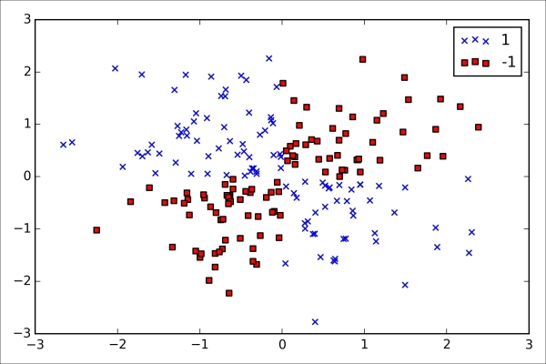
Obviously, we would not be able to separate samples from the positive and negative class very well using a linear hyperplane as the decision boundary via the linear logistic regression or linear SVM model that we discussed in earlier sections.
The basic idea behind kernel methods to deal with such linearly inseparable data is to create nonlinear combinations of the original features to project them onto a higher dimensional space via a mapping function  where it becomes linearly separable. As shown in the next figure, we can transform a two-dimensional dataset onto a new three-dimensional feature space where the classes become separable via the following projection:
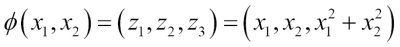
This allows us to separate the two classes shown in the plot via a linear hyperplane that becomes a nonlinear decision boundary if we project it back onto the original feature space:
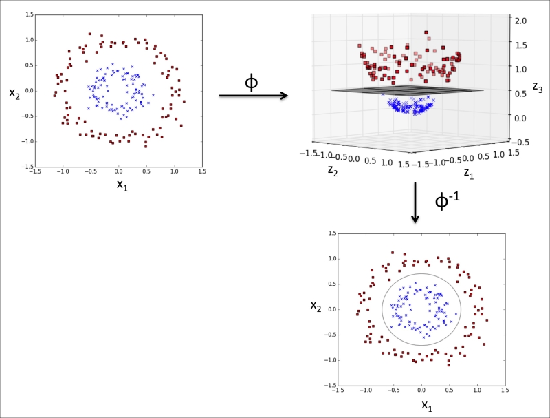
To solve a nonlinear problem using an SVM, we transform the training data onto a higher dimensional feature space via a mapping function and train a linear SVM model to classify the data in this new feature space. Then we can use the same mapping function to transform new, unseen data to classify it using the linear SVM model.
However, one problem with this mapping approach is that the construction of the new features is computationally very expensive, especially if we are dealing with high-dimensional data. This is where the so-called kernel trick comes into play. Although we didn't go into much detail about how to solve the quadratic programming task to train an SVM, in practice all we need is to replace the dot product  by
by  . In order to save the expensive step of calculating this dot product between two points explicitly, we define a so-called kernel function:
  =
=  .
.
One of the most widely used kernels is the Radial Basis Function kernel (RBF kernel) or Gaussian kernel:
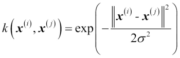
This is often simplified to:
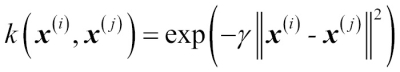
Here,  is a free parameter that is to be optimized.
Roughly speaking, the term kernel can be interpreted as a similarity function between a pair of samples. The minus sign inverts the distance measure into a similarity score and, due to the exponential term, the resulting similarity score will fall into a range between 1 (for exactly similar samples) and 0 (for very dissimilar samples).
Now that we defined the big picture behind the kernel trick, let's see if we can train a kernel SVM that is able to draw a nonlinear decision boundary that separates the XOR data well. Here, we simply use the SVC class from scikit-learn that we imported earlier and replace the parameter kernel='linear' with kernel='rbf':
>>> svm = SVC(kernel='rbf', random_state=0, gamma=0.10, C=10.0) >>> svm.fit(X_xor, y_xor) >>> plot_decision_regions(X_xor, y_xor, classifier=svm) >>> plt.legend(loc='upper left') >>> plt.show()
As we can see in the resulting plot, the kernel SVM separates the XOR data relatively well:
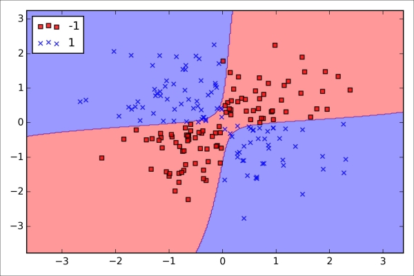
The  parameter, which we set to
 gamma=0.1, can be understood as a cut-off parameter for the Gaussian sphere. If we increase the value for , we increase the influence or reach of the training samples, which leads to a softer decision boundary. To get a better intuition for , let's apply RBF kernel SVM to our Iris flower dataset:
>>> svm = SVC(kernel='rbf', random_state=0, gamma=0.2, C=1.0)
>>> svm.fit(X_train_std, y_train)
>>> plot_decision_regions(X_combined_std,
... y_combined, classifier=svm,
... test_idx=range(105,150))
>>> plt.xlabel('petal length [standardized]')
>>> plt.ylabel('petal width [standardized]')
>>> plt.legend(loc='upper left')
>>> plt.show()Since we chose a relatively small value for , the resulting decision boundary of the RBF kernel SVM model will be relatively soft, as shown in the following figure:
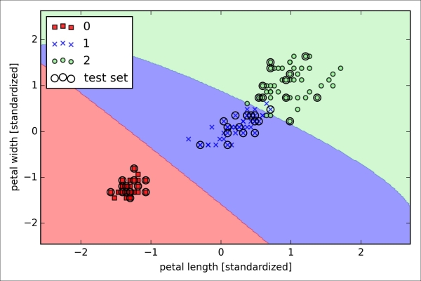
Now let's increase the value of and observe the effect on the decision boundary:
>>> svm = SVC(kernel='rbf', random_state=0, gamma=100.0, C=1.0)
>>> svm.fit(X_train_std, y_train)
>>> plot_decision_regions(X_combined_std,
... y_combined, classifier=svm,
... test_idx=range(105,150))
>>> plt.xlabel('petal length [standardized]')
>>> plt.ylabel('petal width [standardized]')
>>> plt.legend(loc='upper left')
>>> plt.show()In the resulting plot, we can now see that the decision boundary around the classes 0 and 1 is much tighter using a relatively large value of :
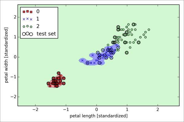
Although the model fits the training dataset very well, such a classifier will likely have a high generalization error on unseen data, which illustrates that the optimization of also plays an important role in controlling overfitting.
Using the kernel trick to find separating hyperplanes in higher dimensional space
To solve a nonlinear problem using an SVM, we transform the training data onto a higher dimensional feature space via a mapping function and train a linear SVM model to classify the data in this new feature space. Then we can use the same mapping function to transform new, unseen data to classify it using the linear SVM model.
However, one problem with this mapping approach is that the construction of the new features is computationally very expensive, especially if we are dealing with high-dimensional data. This is where the so-called kernel trick comes into play. Although we didn't go into much detail about how to solve the quadratic programming task to train an SVM, in practice all we need is to replace the dot product by . In order to save the expensive step of calculating this dot product between two points explicitly, we define a so-called kernel function: = .
One of the most widely used kernels is the Radial Basis Function kernel (RBF kernel) or Gaussian kernel:
This is often simplified to:
Here, is a free parameter that is to be optimized.
Roughly speaking, the term kernel can be interpreted as a similarity function between a pair of samples. The minus sign inverts the distance measure into a similarity score and, due to the exponential term, the resulting similarity score will fall into a range between 1 (for exactly similar samples) and 0 (for very dissimilar samples).
Now that we defined the big picture behind the kernel trick, let's see if we can train a kernel SVM that is able to draw a nonlinear decision boundary that separates the XOR data well. Here, we simply use the SVC class from scikit-learn that we imported earlier and replace the parameter kernel='linear' with kernel='rbf':
>>> svm = SVC(kernel='rbf', random_state=0, gamma=0.10, C=10.0) >>> svm.fit(X_xor, y_xor) >>> plot_decision_regions(X_xor, y_xor, classifier=svm) >>> plt.legend(loc='upper left') >>> plt.show()
As we can see in the resulting plot, the kernel SVM separates the XOR data relatively well:
The parameter, which we set to gamma=0.1, can be understood as a cut-off parameter for the Gaussian sphere. If we increase the value for , we increase the influence or reach of the training samples, which leads to a softer decision boundary. To get a better intuition for , let's apply RBF kernel SVM to our Iris flower dataset:
>>> svm = SVC(kernel='rbf', random_state=0, gamma=0.2, C=1.0)
>>> svm.fit(X_train_std, y_train)
>>> plot_decision_regions(X_combined_std,
... y_combined, classifier=svm,
... test_idx=range(105,150))
>>> plt.xlabel('petal length [standardized]')
>>> plt.ylabel('petal width [standardized]')
>>> plt.legend(loc='upper left')
>>> plt.show()Since we chose a relatively small value for , the resulting decision boundary of the RBF kernel SVM model will be relatively soft, as shown in the following figure:
Now let's increase the value of and observe the effect on the decision boundary:
>>> svm = SVC(kernel='rbf', random_state=0, gamma=100.0, C=1.0)
>>> svm.fit(X_train_std, y_train)
>>> plot_decision_regions(X_combined_std,
... y_combined, classifier=svm,
... test_idx=range(105,150))
>>> plt.xlabel('petal length [standardized]')
>>> plt.ylabel('petal width [standardized]')
>>> plt.legend(loc='upper left')
>>> plt.show()In the resulting plot, we can now see that the decision boundary around the classes 0 and 1 is much tighter using a relatively large value of :
Although the model fits the training dataset very well, such a classifier will likely have a high generalization error on unseen data, which illustrates that the optimization of also plays an important role in controlling overfitting.
Decision tree classifiers are attractive models if we care about interpretability. Like the name decision tree suggests, we can think of this model as breaking down our data by making decisions based on asking a series of questions.
Let's consider the following example where we use a decision tree to decide upon an activity on a particular day:
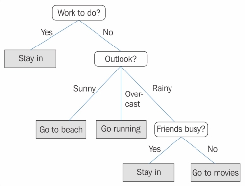
Based on the features in our training set, the decision tree model learns a series of questions to infer the class labels of the samples. Although the preceding figure illustrated the concept of a decision tree based on categorical variables, the same concept applies if our features. This also works if our features are real numbers like in the Iris dataset. For example, we could simply define a cut-off value along the sepal width feature axis and ask a binary question "sepal width  cm?"
cm?"
Using the decision algorithm, we start at the tree root and split the data on the feature that results in the largest information gain (IG), which will be explained in more detail in the following section. In an iterative process, we can then repeat this splitting procedure at each child node until the leaves are pure. This means that the samples at each node all belong to the same class. In practice, this can result in a very deep tree with many nodes, which can easily lead to overfitting. Thus, we typically want to prune the tree by setting a limit for the maximal depth of the tree.
In order to split the nodes at the most informative features, we need to define an objective function that we want to optimize via the tree learning algorithm. Here, our objective function is to maximize the information gain at each split, which we define as follows:
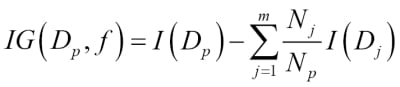
Here, f is the feature to perform the split,  and
and  are the dataset of the parent and jth child node, I is our impurity measure,
  is the total number of samples at the parent node, and
  is the number of samples in the jth child node. As we can see, the information gain is simply the difference between the impurity of the parent node and the sum of the child node impurities—the lower the impurity of the child nodes, the larger the information gain. However, for simplicity and to reduce the combinatorial search space, most libraries (including scikit-learn) implement binary decision trees. This means that each parent node is split into two child nodes,
  and
and  :
:
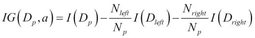
Now, the three impurity measures or splitting criteria that are commonly used in binary decision trees are
Gini index ( ),
entropy (
),
entropy ( ), and the
classification error (
), and the
classification error ( ). Let's start with the definition of entropy for all
non-empty classes (
). Let's start with the definition of entropy for all
non-empty classes ( ):
):
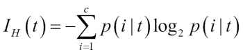
Here,  is the proportion of the samples that belongs to class c for a particular node t. The entropy is therefore 0 if all samples at a node belong to the same class, and the entropy is maximal if we have a uniform class distribution. For example, in a binary class setting, the entropy is 0 if
  or
or  . If the classes are distributed uniformly with
  and
and  , the entropy is 1. Therefore, we can say that the entropy criterion attempts to maximize the mutual information in the tree.
Intuitively, the Gini index can be understood as a criterion to minimize the probability of misclassification:
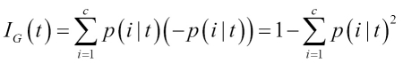
Similar to entropy, the Gini index is maximal if the classes are perfectly mixed, for example, in a binary class setting ( ):
):
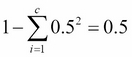
However, in practice both the Gini index and entropy typically yield very similar results and it is often not worth spending much time on evaluating trees using different impurity criteria rather than experimenting with different pruning cut-offs.
Another impurity measure is the classification error:
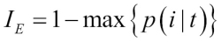
This is a useful criterion for pruning but not recommended for growing a decision tree, since it is less sensitive to changes in the class probabilities of the nodes. We can illustrate this by looking at the two possible splitting scenarios shown in the following figure:
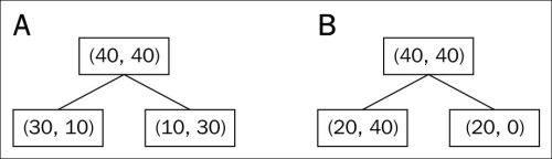
We start with a dataset at the parent node that consists of 40 samples from class 1 and 40 samples from class 2 that we split into two datasets and , respectively. The information gain using the classification error as a splitting criterion would be the same ( ) in both scenario A and B:
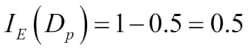
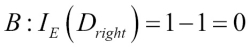
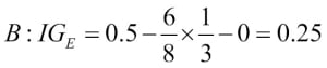
However, the Gini index would favor the split in scenario  over scenario
  , which is indeed more pure:
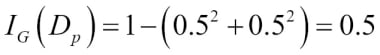
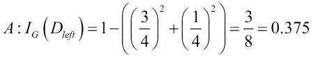
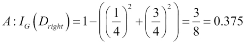
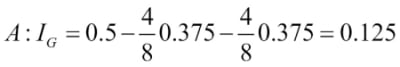
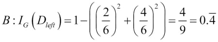
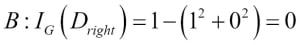
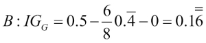
Similarly, the entropy criterion would favor scenario  over scenario
  :
:

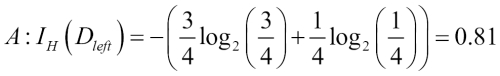
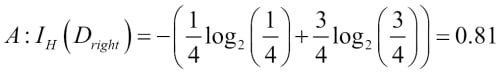
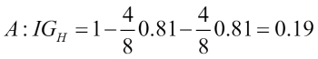
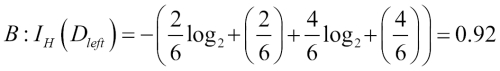
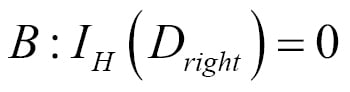
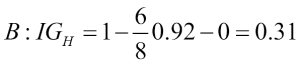
For a more visual comparison of the three different impurity criteria that we discussed previously, let's plot the impurity indices for the probability range [0, 1] for class 1. Note that we will also add in a scaled version of the entropy (entropy/2) to observe that the Gini index is an intermediate measure between entropy and the classification error. The code is as follows:
>>> import matplotlib.pyplot as plt
>>> import numpy as np
>>> def gini(p):
... return (p)*(1 - (p)) + (1 - p)*(1 - (1-p))
>>> def entropy(p):
... return - p*np.log2(p) - (1 - p)*np.log2((1 - p))
>>> def error(p):
... return 1 - np.max([p, 1 - p])
>>> x = np.arange(0.0, 1.0, 0.01)
>>> ent = [entropy(p) if p != 0 else None for p in x]
>>> sc_ent = [e*0.5 if e else None for e in ent]
>>> err = [error(i) for i in x]
>>> fig = plt.figure()
>>> ax = plt.subplot(111)
>>> for i, lab, ls, c, in zip([ent, sc_ent, gini(x), err],
... ['Entropy', 'Entropy (scaled)',
... 'Gini Impurity',
... 'Misclassification Error'],
... ['-', '-', '--', '-.'],
... ['black', 'lightgray',
... 'red', 'green', 'cyan']):
... line = ax.plot(x, i, label=lab,
... linestyle=ls, lw=2, color=c)
>>> ax.legend(loc='upper center', bbox_to_anchor=(0.5, 1.15),
... ncol=3, fancybox=True, shadow=False)
>>> ax.axhline(y=0.5, linewidth=1, color='k', linestyle='--')
>>> ax.axhline(y=1.0, linewidth=1, color='k', linestyle='--')
>>> plt.ylim([0, 1.1])
>>> plt.xlabel('p(i=1)')
>>> plt.ylabel('Impurity Index')
>>> plt.show()The plot produced by the preceding code example is as follows:
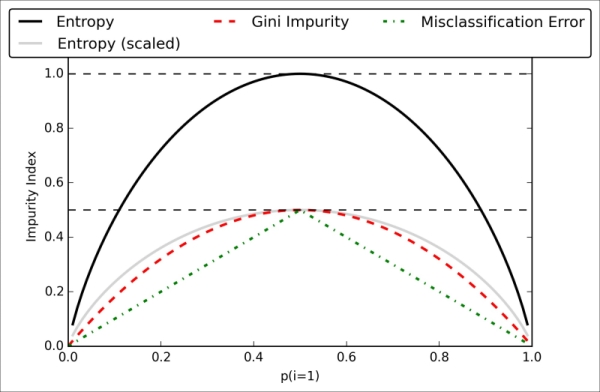
Decision trees can build complex decision boundaries by dividing the feature space into rectangles. However, we have to be careful since the deeper the decision tree, the more complex the decision boundary becomes, which can easily result in overfitting. Using scikit-learn, we will now train a decision tree with a maximum depth of 3 using entropy as a criterion for impurity. Although feature scaling may be desired for visualization purposes, note that feature scaling is not a requirement for decision tree algorithms. The code is as follows:
>>> from sklearn.tree import DecisionTreeClassifier
>>> tree = DecisionTreeClassifier(criterion='entropy',
... max_depth=3, random_state=0)
>>> tree.fit(X_train, y_train)
>>> X_combined = np.vstack((X_train, X_test))
>>> y_combined = np.hstack((y_train, y_test))
>>> plot_decision_regions(X_combined, y_combined,
... classifier=tree, test_idx=range(105,150))
>>>plt.xlabel('petal length [cm]')
>>>plt.ylabel('petal width [cm]')
>>> plt.legend(loc='upper left')
>>> plt.show()After executing the preceding code example, we get the typical axis-parallel decision boundaries of the decision tree:
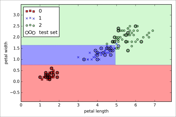
A nice feature in scikit-learn is that it allows us to export the decision tree as a .dot file after training, which we can visualize using the GraphViz program. This program is freely available at http://www.graphviz.org and supported by Linux, Windows, and Mac OS X.
First, we create the .dot file via scikit-learn using the export_graphviz function from the tree submodule, as follows:
>>> from sklearn.tree import export_graphviz >>> export_graphviz(tree, ... out_file='tree.dot', ... feature_names=['petal length', 'petal width'])
After we have installed GraphViz on our computer, we can convert the tree.dot file into a PNG file by executing the following command from the command line in the location where we saved the tree.dot file:
> dot -Tpng tree.dot -o tree.png
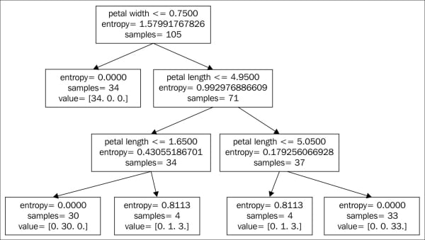
Looking at the decision tree figure that we created via GraphViz, we can now nicely trace back the splits that the decision tree determined from our training dataset. We started with 105 samples at the root and split it into two child nodes with 34 and 71 samples each using the petal with cut-off ≤ 0.75 cm. After the first split, we can see that the left child node is already pure and only contains samples from the Iris-Setosa class (entropy = 0). The further splits on the right are then used to separate the samples from the Iris-Versicolor and Iris-Virginica classes.
Random forests have gained huge popularity in applications of machine learning during the last decade due to their good classification performance, scalability, and ease of use. Intuitively, a random forest can be considered as an ensemble of decision trees. The idea behind ensemble learning is to combine weak learners to build a more robust model, a strong learner, that has a better generalization error and is less susceptible to overfitting. The random forest algorithm can be summarized in four simple steps:
- Draw a random bootstrap sample of size n (randomly choose n samples from the training set with replacement).
- Grow a decision tree from the bootstrap sample. At each node:
- Randomly select d features without replacement.
- Split the node using the feature that provides the best split according to the objective function, for instance, by maximizing the information gain.
- Repeat the steps 1 to 2 k times.
- Aggregate the prediction by each tree to assign the class label by majority vote. Majority voting will be discussed in more detail in Chapter 7, Combining Different Models for Ensemble Learning.
There is a slight modification in step 2 when we are training the individual decision trees: instead of evaluating all features to determine the best split at each node, we only consider a random subset of those.
Although random forests don't offer the same level of interpretability as decision trees, a big advantage of random forests is that we don't have to worry so much about choosing good hyperparameter values. We typically don't need to prune the random forest since the ensemble model is quite robust to noise from the individual decision trees. The only parameter that we really need to care about in practice is the number of trees k (step 3) that we choose for the random forest. Typically, the larger the number of trees, the better the performance of the random forest classifier at the expense of an increased computational cost.
Although it is less common in practice, other hyperparameters of the random forest classifier that can be optimized—using techniques we will discuss in Chapter 5, Compressing Data via Dimensionality Reduction—are the size n of the bootstrap sample (step 1) and the number of features d that is randomly chosen for each split (step 2.1), respectively. Via the sample size n of the bootstrap sample, we control the bias-variance tradeoff of the random forest. By choosing a larger value for n, we decrease the randomness and thus the forest is more likely to overfit. On the other hand, we can reduce the degree of overfitting by choosing smaller values for n at the expense of the model performance. In most implementations, including the RandomForestClassifier implementation in scikit-learn, the sample size of the bootstrap sample is chosen to be equal to the number of samples in the original training set, which usually provides a good bias-variance tradeoff. For the number of features d at each split, we want to choose a value that is smaller than the total number of features in the training set. A reasonable default that is used in scikit-learn and other implementations is  , where m is the number of features in the training set.
Conveniently, we don't have to construct the random forest classifier from individual decision trees by ourselves; there is already an implementation in scikit-learn that we can use:
>>> from sklearn.ensemble import RandomForestClassifier
>>> forest = RandomForestClassifier(criterion='entropy',
... n_estimators=10,
... random_state=1,
... n_jobs=2)
>>> forest.fit(X_train, y_train)
>>> plot_decision_regions(X_combined, y_combined,
... classifier=forest, test_idx=range(105,150))
>>> plt.xlabel('petal length')
>>> plt.ylabel('petal width')
>>> plt.legend(loc='upper left')
>>> plt.show()After executing the preceding code, we should see the decision regions formed by the ensemble of trees in the random forest, as shown in the following figure:
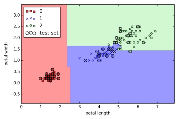
Using the preceding code, we trained a random forest from 10 decision trees via the n_estimators parameter and used the entropy criterion as an impurity measure to split the nodes. Although we are growing a very small random forest from a very small training dataset, we used the n_jobs parameter for demonstration purposes, which allows us to parallelize the model training using multiple cores of our computer (here, two).
Maximizing information gain – getting the most bang for the buck
In order to split the nodes at the most informative features, we need to define an objective function that we want to optimize via the tree learning algorithm. Here, our objective function is to maximize the information gain at each split, which we define as follows:
Here, f is the feature to perform the split, and are the dataset of the parent and jth child node, I is our impurity measure, is the total number of samples at the parent node, and is the number of samples in the jth child node. As we can see, the information gain is simply the difference between the impurity of the parent node and the sum of the child node impurities—the lower the impurity of the child nodes, the larger the information gain. However, for simplicity and to reduce the combinatorial search space, most libraries (including scikit-learn) implement binary decision trees. This means that each parent node is split into two child nodes, and :
Now, the three impurity measures or splitting criteria that are commonly used in binary decision trees are
Gini index (),
entropy (), and the
classification error (). Let's start with the definition of entropy for all
non-empty classes ():
Here, is the proportion of the samples that belongs to class c for a particular node t. The entropy is therefore 0 if all samples at a node belong to the same class, and the entropy is maximal if we have a uniform class distribution. For example, in a binary class setting, the entropy is 0 if or . If the classes are distributed uniformly with and , the entropy is 1. Therefore, we can say that the entropy criterion attempts to maximize the mutual information in the tree.
Intuitively, the Gini index can be understood as a criterion to minimize the probability of misclassification:
Similar to entropy, the Gini index is maximal if the classes are perfectly mixed, for example, in a binary class setting ():
However, in practice both the Gini index and entropy typically yield very similar results and it is often not worth spending much time on evaluating trees using different impurity criteria rather than experimenting with different pruning cut-offs.
Another impurity measure is the classification error:
This is a useful criterion for pruning but not recommended for growing a decision tree, since it is less sensitive to changes in the class probabilities of the nodes. We can illustrate this by looking at the two possible splitting scenarios shown in the following figure:
We start with a dataset at the parent node that consists of 40 samples from class 1 and 40 samples from class 2 that we split into two datasets and , respectively. The information gain using the classification error as a splitting criterion would be the same () in both scenario A and B:
However, the Gini index would favor the split in scenario over scenario , which is indeed more pure:
Similarly, the entropy criterion would favor scenario over scenario :
For a more visual comparison of the three different impurity criteria that we discussed previously, let's plot the impurity indices for the probability range [0, 1] for class 1. Note that we will also add in a scaled version of the entropy (entropy/2) to observe that the Gini index is an intermediate measure between entropy and the classification error. The code is as follows:
>>> import matplotlib.pyplot as plt
>>> import numpy as np
>>> def gini(p):
... return (p)*(1 - (p)) + (1 - p)*(1 - (1-p))
>>> def entropy(p):
... return - p*np.log2(p) - (1 - p)*np.log2((1 - p))
>>> def error(p):
... return 1 - np.max([p, 1 - p])
>>> x = np.arange(0.0, 1.0, 0.01)
>>> ent = [entropy(p) if p != 0 else None for p in x]
>>> sc_ent = [e*0.5 if e else None for e in ent]
>>> err = [error(i) for i in x]
>>> fig = plt.figure()
>>> ax = plt.subplot(111)
>>> for i, lab, ls, c, in zip([ent, sc_ent, gini(x), err],
... ['Entropy', 'Entropy (scaled)',
... 'Gini Impurity',
... 'Misclassification Error'],
... ['-', '-', '--', '-.'],
... ['black', 'lightgray',
... 'red', 'green', 'cyan']):
... line = ax.plot(x, i, label=lab,
... linestyle=ls, lw=2, color=c)
>>> ax.legend(loc='upper center', bbox_to_anchor=(0.5, 1.15),
... ncol=3, fancybox=True, shadow=False)
>>> ax.axhline(y=0.5, linewidth=1, color='k', linestyle='--')
>>> ax.axhline(y=1.0, linewidth=1, color='k', linestyle='--')
>>> plt.ylim([0, 1.1])
>>> plt.xlabel('p(i=1)')
>>> plt.ylabel('Impurity Index')
>>> plt.show()The plot produced by the preceding code example is as follows:
Decision trees can build complex decision boundaries by dividing the feature space into rectangles. However, we have to be careful since the deeper the decision tree, the more complex the decision boundary becomes, which can easily result in overfitting. Using scikit-learn, we will now train a decision tree with a maximum depth of 3 using entropy as a criterion for impurity. Although feature scaling may be desired for visualization purposes, note that feature scaling is not a requirement for decision tree algorithms. The code is as follows:
>>> from sklearn.tree import DecisionTreeClassifier
>>> tree = DecisionTreeClassifier(criterion='entropy',
... max_depth=3, random_state=0)
>>> tree.fit(X_train, y_train)
>>> X_combined = np.vstack((X_train, X_test))
>>> y_combined = np.hstack((y_train, y_test))
>>> plot_decision_regions(X_combined, y_combined,
... classifier=tree, test_idx=range(105,150))
>>>plt.xlabel('petal length [cm]')
>>>plt.ylabel('petal width [cm]')
>>> plt.legend(loc='upper left')
>>> plt.show()After executing the preceding code example, we get the typical axis-parallel decision boundaries of the decision tree:
A nice feature in scikit-learn is that it allows us to export the decision tree as a .dot file after training, which we can visualize using the GraphViz program. This program is freely available at http://www.graphviz.org and supported by Linux, Windows, and Mac OS X.
First, we create the .dot file via scikit-learn using the export_graphviz function from the tree submodule, as follows:
>>> from sklearn.tree import export_graphviz >>> export_graphviz(tree, ... out_file='tree.dot', ... feature_names=['petal length', 'petal width'])
After we have installed GraphViz on our computer, we can convert the tree.dot file into a PNG file by executing the following command from the command line in the location where we saved the tree.dot file:
> dot -Tpng tree.dot -o tree.png
Looking at the decision tree figure that we created via GraphViz, we can now nicely trace back the splits that the decision tree determined from our training dataset. We started with 105 samples at the root and split it into two child nodes with 34 and 71 samples each using the petal with cut-off ≤ 0.75 cm. After the first split, we can see that the left child node is already pure and only contains samples from the Iris-Setosa class (entropy = 0). The further splits on the right are then used to separate the samples from the Iris-Versicolor and Iris-Virginica classes.
Random forests have gained huge popularity in applications of machine learning during the last decade due to their good classification performance, scalability, and ease of use. Intuitively, a random forest can be considered as an ensemble of decision trees. The idea behind ensemble learning is to combine weak learners to build a more robust model, a strong learner, that has a better generalization error and is less susceptible to overfitting. The random forest algorithm can be summarized in four simple steps:
- Draw a random bootstrap sample of size n (randomly choose n samples from the training set with replacement).
- Grow a decision tree from the bootstrap sample. At each node:
- Randomly select d features without replacement.
- Split the node using the feature that provides the best split according to the objective function, for instance, by maximizing the information gain.
- Repeat the steps 1 to 2 k times.
- Aggregate the prediction by each tree to assign the class label by majority vote. Majority voting will be discussed in more detail in Chapter 7, Combining Different Models for Ensemble Learning.
There is a slight modification in step 2 when we are training the individual decision trees: instead of evaluating all features to determine the best split at each node, we only consider a random subset of those.
Although random forests don't offer the same level of interpretability as decision trees, a big advantage of random forests is that we don't have to worry so much about choosing good hyperparameter values. We typically don't need to prune the random forest since the ensemble model is quite robust to noise from the individual decision trees. The only parameter that we really need to care about in practice is the number of trees k (step 3) that we choose for the random forest. Typically, the larger the number of trees, the better the performance of the random forest classifier at the expense of an increased computational cost.
Although it is less common in practice, other hyperparameters of the random forest classifier that can be optimized—using techniques we will discuss in Chapter 5, Compressing Data via Dimensionality Reduction—are the size n of the bootstrap sample (step 1) and the number of features d that is randomly chosen for each split (step 2.1), respectively. Via the sample size n of the bootstrap sample, we control the bias-variance tradeoff of the random forest. By choosing a larger value for n, we decrease the randomness and thus the forest is more likely to overfit. On the other hand, we can reduce the degree of overfitting by choosing smaller values for n at the expense of the model performance. In most implementations, including the RandomForestClassifier implementation in scikit-learn, the sample size of the bootstrap sample is chosen to be equal to the number of samples in the original training set, which usually provides a good bias-variance tradeoff. For the number of features d at each split, we want to choose a value that is smaller than the total number of features in the training set. A reasonable default that is used in scikit-learn and other implementations is , where m is the number of features in the training set.
Conveniently, we don't have to construct the random forest classifier from individual decision trees by ourselves; there is already an implementation in scikit-learn that we can use:
>>> from sklearn.ensemble import RandomForestClassifier
>>> forest = RandomForestClassifier(criterion='entropy',
... n_estimators=10,
... random_state=1,
... n_jobs=2)
>>> forest.fit(X_train, y_train)
>>> plot_decision_regions(X_combined, y_combined,
... classifier=forest, test_idx=range(105,150))
>>> plt.xlabel('petal length')
>>> plt.ylabel('petal width')
>>> plt.legend(loc='upper left')
>>> plt.show()After executing the preceding code, we should see the decision regions formed by the ensemble of trees in the random forest, as shown in the following figure:
Using the preceding code, we trained a random forest from 10 decision trees via the n_estimators parameter and used the entropy criterion as an impurity measure to split the nodes. Although we are growing a very small random forest from a very small training dataset, we used the n_jobs parameter for demonstration purposes, which allows us to parallelize the model training using multiple cores of our computer (here, two).
Building a decision tree
Decision trees can build complex decision boundaries by dividing the feature space into rectangles. However, we have to be careful since the deeper the decision tree, the more complex the decision boundary becomes, which can easily result in overfitting. Using scikit-learn, we will now train a decision tree with a maximum depth of 3 using entropy as a criterion for impurity. Although feature scaling may be desired for visualization purposes, note that feature scaling is not a requirement for decision tree algorithms. The code is as follows:
>>> from sklearn.tree import DecisionTreeClassifier
>>> tree = DecisionTreeClassifier(criterion='entropy',
... max_depth=3, random_state=0)
>>> tree.fit(X_train, y_train)
>>> X_combined = np.vstack((X_train, X_test))
>>> y_combined = np.hstack((y_train, y_test))
>>> plot_decision_regions(X_combined, y_combined,
... classifier=tree, test_idx=range(105,150))
>>>plt.xlabel('petal length [cm]')
>>>plt.ylabel('petal width [cm]')
>>> plt.legend(loc='upper left')
>>> plt.show()After executing the preceding code example, we get the typical axis-parallel decision boundaries of the decision tree:
A nice feature in scikit-learn is that it allows us to export the decision tree as a .dot file after training, which we can visualize using the GraphViz program. This program is freely available at http://www.graphviz.org and supported by Linux, Windows, and Mac OS X.
First, we create the .dot file via scikit-learn using the export_graphviz function from the tree submodule, as follows:
>>> from sklearn.tree import export_graphviz >>> export_graphviz(tree, ... out_file='tree.dot', ... feature_names=['petal length', 'petal width'])
After we have installed GraphViz on our computer, we can convert the tree.dot file into a PNG file by executing the following command from the command line in the location where we saved the tree.dot file:
> dot -Tpng tree.dot -o tree.png
Looking at the decision tree figure that we created via GraphViz, we can now nicely trace back the splits that the decision tree determined from our training dataset. We started with 105 samples at the root and split it into two child nodes with 34 and 71 samples each using the petal with cut-off ≤ 0.75 cm. After the first split, we can see that the left child node is already pure and only contains samples from the Iris-Setosa class (entropy = 0). The further splits on the right are then used to separate the samples from the Iris-Versicolor and Iris-Virginica classes.
Random forests have gained huge popularity in applications of machine learning during the last decade due to their good classification performance, scalability, and ease of use. Intuitively, a random forest can be considered as an ensemble of decision trees. The idea behind ensemble learning is to combine weak learners to build a more robust model, a strong learner, that has a better generalization error and is less susceptible to overfitting. The random forest algorithm can be summarized in four simple steps:
- Draw a random bootstrap sample of size n (randomly choose n samples from the training set with replacement).
- Grow a decision tree from the bootstrap sample. At each node:
- Randomly select d features without replacement.
- Split the node using the feature that provides the best split according to the objective function, for instance, by maximizing the information gain.
- Repeat the steps 1 to 2 k times.
- Aggregate the prediction by each tree to assign the class label by majority vote. Majority voting will be discussed in more detail in Chapter 7, Combining Different Models for Ensemble Learning.
There is a slight modification in step 2 when we are training the individual decision trees: instead of evaluating all features to determine the best split at each node, we only consider a random subset of those.
Although random forests don't offer the same level of interpretability as decision trees, a big advantage of random forests is that we don't have to worry so much about choosing good hyperparameter values. We typically don't need to prune the random forest since the ensemble model is quite robust to noise from the individual decision trees. The only parameter that we really need to care about in practice is the number of trees k (step 3) that we choose for the random forest. Typically, the larger the number of trees, the better the performance of the random forest classifier at the expense of an increased computational cost.
Although it is less common in practice, other hyperparameters of the random forest classifier that can be optimized—using techniques we will discuss in Chapter 5, Compressing Data via Dimensionality Reduction—are the size n of the bootstrap sample (step 1) and the number of features d that is randomly chosen for each split (step 2.1), respectively. Via the sample size n of the bootstrap sample, we control the bias-variance tradeoff of the random forest. By choosing a larger value for n, we decrease the randomness and thus the forest is more likely to overfit. On the other hand, we can reduce the degree of overfitting by choosing smaller values for n at the expense of the model performance. In most implementations, including the RandomForestClassifier implementation in scikit-learn, the sample size of the bootstrap sample is chosen to be equal to the number of samples in the original training set, which usually provides a good bias-variance tradeoff. For the number of features d at each split, we want to choose a value that is smaller than the total number of features in the training set. A reasonable default that is used in scikit-learn and other implementations is , where m is the number of features in the training set.
Conveniently, we don't have to construct the random forest classifier from individual decision trees by ourselves; there is already an implementation in scikit-learn that we can use:
>>> from sklearn.ensemble import RandomForestClassifier
>>> forest = RandomForestClassifier(criterion='entropy',
... n_estimators=10,
... random_state=1,
... n_jobs=2)
>>> forest.fit(X_train, y_train)
>>> plot_decision_regions(X_combined, y_combined,
... classifier=forest, test_idx=range(105,150))
>>> plt.xlabel('petal length')
>>> plt.ylabel('petal width')
>>> plt.legend(loc='upper left')
>>> plt.show()After executing the preceding code, we should see the decision regions formed by the ensemble of trees in the random forest, as shown in the following figure:
Using the preceding code, we trained a random forest from 10 decision trees via the n_estimators parameter and used the entropy criterion as an impurity measure to split the nodes. Although we are growing a very small random forest from a very small training dataset, we used the n_jobs parameter for demonstration purposes, which allows us to parallelize the model training using multiple cores of our computer (here, two).
Combining weak to strong learners via random forests
Random forests have gained huge popularity in applications of machine learning during the last decade due to their good classification performance, scalability, and ease of use. Intuitively, a random forest can be considered as an ensemble of decision trees. The idea behind ensemble learning is to combine weak learners to build a more robust model, a strong learner, that has a better generalization error and is less susceptible to overfitting. The random forest algorithm can be summarized in four simple steps:
- Draw a random bootstrap sample of size n (randomly choose n samples from the training set with replacement).
- Grow a decision tree from the bootstrap sample. At each node:
- Randomly select d features without replacement.
- Split the node using the feature that provides the best split according to the objective function, for instance, by maximizing the information gain.
- Repeat the steps 1 to 2 k times.
- Aggregate the prediction by each tree to assign the class label by majority vote. Majority voting will be discussed in more detail in Chapter 7, Combining Different Models for Ensemble Learning.
There is a slight modification in step 2 when we are training the individual decision trees: instead of evaluating all features to determine the best split at each node, we only consider a random subset of those.
Although random forests don't offer the same level of interpretability as decision trees, a big advantage of random forests is that we don't have to worry so much about choosing good hyperparameter values. We typically don't need to prune the random forest since the ensemble model is quite robust to noise from the individual decision trees. The only parameter that we really need to care about in practice is the number of trees k (step 3) that we choose for the random forest. Typically, the larger the number of trees, the better the performance of the random forest classifier at the expense of an increased computational cost.
Although it is less common in practice, other hyperparameters of the random forest classifier that can be optimized—using techniques we will discuss in Chapter 5, Compressing Data via Dimensionality Reduction—are the size n of the bootstrap sample (step 1) and the number of features d that is randomly chosen for each split (step 2.1), respectively. Via the sample size n of the bootstrap sample, we control the bias-variance tradeoff of the random forest. By choosing a larger value for n, we decrease the randomness and thus the forest is more likely to overfit. On the other hand, we can reduce the degree of overfitting by choosing smaller values for n at the expense of the model performance. In most implementations, including the RandomForestClassifier implementation in scikit-learn, the sample size of the bootstrap sample is chosen to be equal to the number of samples in the original training set, which usually provides a good bias-variance tradeoff. For the number of features d at each split, we want to choose a value that is smaller than the total number of features in the training set. A reasonable default that is used in scikit-learn and other implementations is , where m is the number of features in the training set.
Conveniently, we don't have to construct the random forest classifier from individual decision trees by ourselves; there is already an implementation in scikit-learn that we can use:
>>> from sklearn.ensemble import RandomForestClassifier
>>> forest = RandomForestClassifier(criterion='entropy',
... n_estimators=10,
... random_state=1,
... n_jobs=2)
>>> forest.fit(X_train, y_train)
>>> plot_decision_regions(X_combined, y_combined,
... classifier=forest, test_idx=range(105,150))
>>> plt.xlabel('petal length')
>>> plt.ylabel('petal width')
>>> plt.legend(loc='upper left')
>>> plt.show()After executing the preceding code, we should see the decision regions formed by the ensemble of trees in the random forest, as shown in the following figure:
Using the preceding code, we trained a random forest from 10 decision trees via the n_estimators parameter and used the entropy criterion as an impurity measure to split the nodes. Although we are growing a very small random forest from a very small training dataset, we used the n_jobs parameter for demonstration purposes, which allows us to parallelize the model training using multiple cores of our computer (here, two).
The last supervised learning algorithm that we want to discuss in this chapter is the k-nearest neighbor classifier (KNN), which is particularly interesting because it is fundamentally different from the learning algorithms that we have discussed so far.
KNN is a typical example of a lazy learner. It is called lazy not because of its apparent simplicity, but because it doesn't learn a discriminative function from the training data but memorizes the training dataset instead.
Note
Parametric versus nonparametric models
Machine learning algorithms can be grouped into parametric and nonparametric models. Using parametric models, we estimate parameters from the training dataset to learn a function that can classify new data points without requiring the original training dataset anymore. Typical examples of parametric models are the perceptron, logistic regression, and the linear SVM. In contrast, nonparametric models can't be characterized by a fixed set of parameters, and the number of parameters grows with the training data. Two examples of nonparametric models that we have seen so far are the decision tree classifier/random forest and the kernel SVM.
KNN belongs to a subcategory of nonparametric models that is described as instance-based learning. Models based on instance-based learning are characterized by memorizing the training dataset, and lazy learning is a special case of instance-based learning that is associated with no (zero) cost during the learning process.
The KNN algorithm itself is fairly straightforward and can be summarized by the following steps:
- Choose the number of k and a distance metric.
- Find the k nearest neighbors of the sample that we want to classify.
- Assign the class label by majority vote.
The following figure illustrates how a new data point (?) is assigned the triangle class label based on majority voting among its five nearest neighbors.
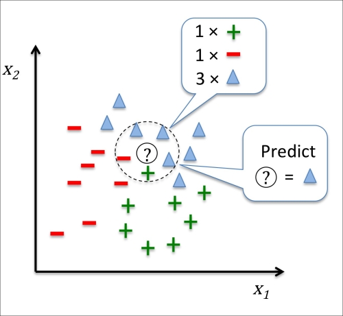
Based on the chosen distance metric, the KNN algorithm finds the k samples in the training dataset that are closest (most similar) to the point that we want to classify. The class label of the new data point is then determined by a majority vote among its k nearest neighbors.
The main advantage of such a memory-based approach is that the classifier immediately adapts as we collect new training data. However, the downside is that the computational complexity for classifying new samples grows linearly with the number of samples in the training dataset in the worst-case scenario—unless the dataset has very few dimensions (features) and the algorithm has been implemented using efficient data structures such as KD-trees. J. H. Friedman, J. L. Bentley, and R. A. Finkel. An algorithm for finding best matches in logarithmic expected time. ACM Transactions on Mathematical Software (TOMS), 3(3):209–226, 1977. Furthermore, we can't discard training samples since no training step is involved. Thus, storage space can become a challenge if we are working with large datasets.
By executing the following code, we will now implement a KNN model in scikit-learn using an Euclidean distance metric:
>>> from sklearn.neighbors import KNeighborsClassifier
>>> knn = KNeighborsClassifier(n_neighbors=5, p=2,
... metric='minkowski')
>>> knn.fit(X_train_std, y_train)
>>> plot_decision_regions(X_combined_std, y_combined,
... classifier=knn, test_idx=range(105,150))
>>> plt.xlabel('petal length [standardized]')
>>> plt.ylabel('petal width [standardized]')
>>> plt.show()By specifying five neighbors in the KNN model for this dataset, we obtain a relatively smooth decision boundary, as shown in the following figure:
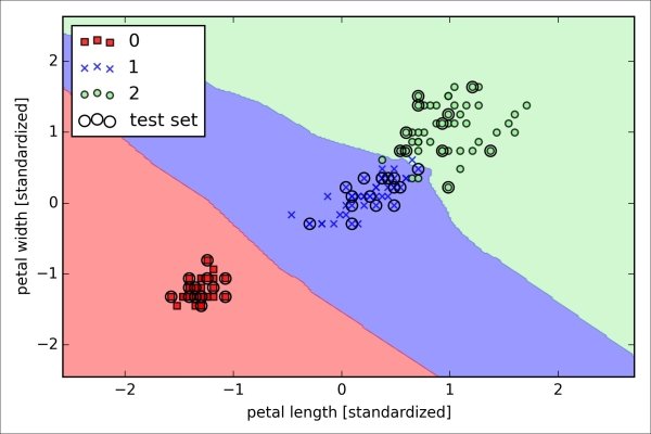
The right choice of k is crucial to find a good balance between over- and underfitting. We also have to make sure that we choose a distance metric that is appropriate for the features in the dataset. Often, a simple Euclidean distance measure is used for real-valued samples, for example, the flowers in our Iris dataset, which have features measured in centimeters. However, if we are using a Euclidean distance measure, it is also important to standardize the data so that each feature contributes equally to the distance. The 'minkowski' distance that we used in the previous code is just a generalization of the Euclidean and Manhattan distance that can be written as follows:
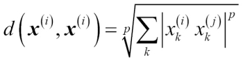
It becomes the Euclidean distance if we set the parameter p=2 or the Manhatten distance at p=1, respectively. Many other distance metrics are available in scikit-learn and can be provided to the metric parameter. They are listed at http://scikit-learn.org/stable/modules/generated/sklearn.neighbors.DistanceMetric.html.
Note
The curse of dimensionality
It is important to mention that KNN is very susceptible to overfitting due to the curse of dimensionality. The curse of dimensionality describes the phenomenon where the feature space becomes increasingly sparse for an increasing number of dimensions of a fixed-size training dataset. Intuitively, we can think of even the closest neighbors being too far away in a high-dimensional space to give a good estimate.
We have discussed the concept of regularization in the section about logistic regression as one way to avoid overfitting. However, in models where regularization is not applicable such as decision trees and KNN, we can use feature selection and dimensionality reduction techniques to help us avoid the curse of dimensionality. This will be discussed in more detail in the next chapter.
In this chapter, you learned about many different machine algorithms that are used to tackle linear and nonlinear problems. We have seen that decision trees are particularly attractive if we care about interpretability. Logistic regression is not only a useful model for online learning via stochastic gradient descent, but also allows us to predict the probability of a particular event. Although support vector machines are powerful linear models that can be extended to nonlinear problems via the kernel trick, they have many parameters that have to be tuned in order to make good predictions. In contrast, ensemble methods such as random forests don't require much parameter tuning and don't overfit so easily as decision trees, which makes it an attractive model for many practical problem domains. The K-nearest neighbor classifier offers an alternative approach to classification via lazy learning that allows us to make predictions without any model training but with a more computationally expensive prediction step.
However, even more important than the choice of an appropriate learning algorithm is the available data in our training dataset. No algorithm will be able to make good predictions without informative and discriminatory features.
In the next chapter, we will discuss important topics regarding the preprocessing of data, feature selection, and dimensionality reduction, which we will need to build powerful machine learning models. Later in Chapter 6, Learning Best Practices for Model Evaluation and Hyperparameter Tuning, we will see how we can evaluate and compare the performance of our models and learn useful tricks to fine-tune the different algorithms.