
In the previous chapter, we went over a lot of mathematical concepts to understand how feedforward artificial neural networks and multilayer perceptrons in particular work. First and foremost, having a good understanding of the mathematical underpinnings of machine learning algorithms is very important, since it helps us to use those powerful algorithms most effectively and correctly. Throughout the previous chapters, you dedicated a lot of time to learning the best practices of machine learning, and you even practiced implementing algorithms yourself from scratch. In this chapter, you can lean back a little bit and rest on your laurels, I want you to enjoy this exciting journey through one of the most powerful libraries that is used by machine learning researchers to experiment with deep neural networks and train them very efficiently. Most of modern machine learning research utilizes computers with powerful Graphics Processing Units (GPUs). If you are interested in diving into deep learning, which is currently the hottest topic in machine learning research, this chapter is definitely for you. However, do not worry if you do not have access to GPUs; in this chapter, the use of GPUs will be optional, not required.
Before we get started, let me give you a brief overview of the topics that we will cover in this chapter:
- Writing optimized machine learning code with Theano
- Choosing activation functions for artificial neural networks
- Using the Keras deep learning library for fast and easy experimentation
In this section, we will explore the powerful Theano tool, which has been designed to train machine learning models most effectively using Python. The Theano development started back in 2008 in the LISA lab (short for Laboratoire d'Informatique des Systèmes Adaptatifs (http://lisa.iro.umontreal.ca)) lead by Yoshua Bengio.
Before we discuss what Theano really is and what it can do for us to speed up our machine learning tasks, let's discuss some of the challenges when we are running expensive calculations on our hardware. Luckily, the performance of computer processors keeps on improving constantly over the years, which allows us to train more powerful and complex learning systems to improve the predictive performance of our machine learning models. Even the cheapest desktop computer hardware that is available nowadays comes with processing units that have multiple cores. In the previous chapters, we saw that many functions in scikit-learn allow us to spread the computations over multiple processing units. However, by default, Python is limited to execution on one core, due to the
Global Interpreter Lock (GIL). However, although we take advantage of its multiprocessing library to distribute computations over multiple cores, we have to consider that even advanced desktop hardware rarely comes with more than 8 or 16 such cores.
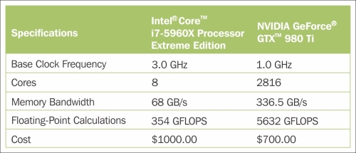
If we think back of the previous chapter where we implemented a very simple multilayer perceptron with only one hidden layer consisting of 50 units, we already had to optimize approximately 1000 weights to learn a model for a very simple image classification task. The images in MNIST are rather small (28 x 28 pixels), and we can only imagine the explosion in the number of parameters if we want to add additional hidden layers or work with images that have higher pixel densities. Such a task would quickly become unfeasible for a single processing unit. Now, the question is how can we tackle such problems more effectively? The obvious solution to this problem is to use GPUs. GPUs are real power horses. You can think of a graphics card as a small computer cluster inside your machine. Another advantage is that modern GPUs are relatively cheap compared to the state-of-the-art CPUs, as we can see in the following overview:
Sources for this can be found on the following websites:
(date: August 20, 2015)
At 70 percent of the price of a modern CPU, we can get a GPU that has 450 times more cores, and is capable of around 15 times more floating-point calculations per second. So, what is holding us back from utilizing GPUs for our machine learning tasks? The challenge is that writing code to target GPUs is not as trivial as executing Python code in our interpreter. There are special packages such as CUDA and OpenCL that allow us to target the GPU. However, writing code in CUDA or OpenCL is probably not the most convenient environment for implementing and running machine learning algorithms. The good news is that this is what Theano was developed for!
What exactly is Theano—a programming language, a compiler, or a Python library? It turns out that it fits all these descriptions. Theano has been developed to implement, compile, and evaluate mathematical expressions very efficiently with a strong focus on multidimensional arrays (tensors). It comes with an option to run code on CPU(s). However, its real power comes from utilizing GPUs to take advantage of the large memory bandwidths and great capabilities for floating point math. Using Theano, we can easily run code in parallel over shared memory as well. In 2010, the developers of Theano reported an 1.8x faster performance than NumPy when the code was run on the CPU, and if Theano targeted the GPU, it was even 11x faster than NumPy (J. Bergstra, O. Breuleux, F. Bastien, P. Lamblin, R. Pascanu, G. Desjardins, J. Turian, D. Warde-Farley, and Y. Bengio. Theano: A CPU and GPU Math Compiler in Python. In Proc. 9th Python in Science Conf, pages 1–7, 2010.). Now, keep in mind that this benchmark is from 2010, and Theano has improved significantly over the years, and so have the capabilities of modern graphics cards.
So, how does Theano relate to NumPy? Theano is built on top of NumPy and it has a very similar syntax, which makes the usage very convenient for people who are already familiar with the latter. To be fair, Theano is not just "NumPy on steroids" as many people would describe it, but it also shares some similarities with SymPy (http://www.sympy.org), a Python package for symbolic computations (or symbolic algebra). As we saw in previous chapters, in NumPy, we describe what our variables are, and how we want to combine them; then, the code is executed line by line. In Theano, however, we write down the problem first and the description of how we want to analyze it. Then, Theano optimizes and compiles code for us using C/C++, or CUDA/OpenCL if we want to run it on the GPU. In order to generate the optimized code for us, Theano needs to know the scope of our problem; think of it as a tree of operations (or a graph of symbolic expressions). Note that Theano is still under active development, and many new features are added and improvements are made on a regular basis. In this chapter, we will explore the basic concepts behind Theano and learn how to use it for machine learning tasks. Since Theano is a large library with many advanced features, it would be impossible to cover all of them in this book. However, I will provide useful links to the excellent online documentation (http://deeplearning.net/software/theano/) if you want to learn more about this library.
In this section, we will take our first steps with Theano. Depending on how your system is set up, you typically can just use the pip installer and install Theano from PyPI by executing the following from your command-line terminal:
pip install Theano
If you should experience problems with the installation procedure, I recommend you to read more about system and platform-specific recommendations that are provided at http://deeplearning.net/software/theano/install.html. Note that all the code in this chapter can be run on your CPU; using the GPU is entirely optional but recommended if you fully want to enjoy the benefits of Theano. If you have a graphics card that supports either CUDA or OpenCL, please refer to the up-to-date tutorial at http://deeplearning.net/software/theano/tutorial/using_gpu.html#using-gpu to set it up appropriately.
At its core, Theano is built around so-called tensors to evaluate symbolic mathematical expressions. Tensors can be understood as a generalization of scalars, vectors, matrices, and so on. More concretely, a scalar can be defined as a rank-0 tensor, a vector as a rank-1 tensor, a matrix as rank-2 tensor, and matrices stacked in a third dimension as rank-3 tensors. As a warm-up exercise, we will start with the use of simple scalars from the Theano tensor module to compute a net input  of a sample point
  in a one dimensional dataset with weight
  and bias
  :
:
The code is as follows:
>>> import theano
>>> from theano import tensor as T
# initialize
>>> x1 = T.scalar()
>>> w1 = T.scalar()
>>> w0 = T.scalar()
>>> z1 = w1 * x1 + w0
# compile
>>> net_input = theano.function(inputs=[w1, x1, w0],
... outputs=z1)
# execute
>>> print('Net input: %.2f' % net_input(2.0, 1.0, 0.5))
Net input: 2.50This was pretty straightforward, right? If we write code in Theano, we just have to follow three simple steps: define the symbols (Variable objects), compile the code, and execute it. In the initialization step, we defined three symbols, x1, w1, and w0, to compute z1. Then, we compiled a function net_input to compute the net input z1.
However, there is one particular detail that deserves special attention if we write Theano code: the type of our variables (dtype). Consider it as a blessing or burden, but in Theano we need to choose whether we want to use 64 or 32 bit integers or floats, which greatly affects the performance of the code. Let's discuss those variable types in more detail in the next section.
Nowadays, no matter whether we run Mac OS X, Linux, or Microsoft Windows, we mainly use software and applications using 64-bit memory addresses. However, if we want to accelerate the evaluation of mathematical expressions on GPUs, we still often rely on the older 32-bit memory addresses. Currently, this is the only supported computing architecture in Theano. In this section, we will see how to configure Theano appropriately. If you are interested in more details about the Theano configuration, please refer to the online documentation at http://deeplearning.net/software/theano/library/config.html.
When we are implementing machine learning algorithms, we are mostly working with floating point numbers. By default, both NumPy and Theano use the double-precision floating-point format (float64). However, it would be really useful to toggle back and forth float64 (CPU), and float32 (GPU) when we are developing Theano code for prototyping on CPU and execution on GPU. For example, to access the default settings for Theano's float variables, we can execute the following code in our Python interpreter:
>>> print(theano.config.floatX) float64
If you have not modified any settings after the installation of Theano, the floating point default should be float64. However, we can simply change it to float32 in our current Python session via the following code:
>>> theano.config.floatX = 'float32'
Note that although the current GPU utilization in Theano requires float32 types, we can use both float64 and float32 on our CPUs. Thus, if you want to change the default settings globally, you can change the settings in your THEANO_FLAGS variable via the command-line (Bash) terminal:
export THEANO_FLAGS=floatX=float32
Alternatively, you can apply these settings only to a particular Python script, by running it as follows:
THEANO_FLAGS=floatX=float32 python your_script.py
So far, we discussed how to set the default floating-point types to get the best bang for the buck on our GPU using Theano. Next, let's discuss the options to toggle between CPU and GPU execution. If we execute the following code, we can check whether we are using CPU or GPU:
>>> print(theano.config.device) cpu
My personal recommendation is to use cpu as default, which makes prototyping and code debugging easier. For example, you can run Theano code on your CPU by executing it a script, as from your command-line terminal:
THEANO_FLAGS=device=cpu,floatX=float64 python your_script.py
However, once we have implemented the code and want to run it most efficiently utilizing our GPU hardware, we can then run it via the following code without making additional modifications to our original code:
THEANO_FLAGS=device=gpu,floatX=float32 python your_script.py
It may also be convenient to create a .theanorc file in your home directory to make these configurations permanent. For example, to always use float32 and the GPU, you can create such a .theanorc file including these settings. The command is as follows:
echo -e "\n[global]\nfloatX=float32\ndevice=gpu\n" >> ~/.theanorc
If you are not operating on a MacOS X or Linux terminal, you can create a .theanorc file manually using your favorite text editor and add the following contents:
[global] floatX=float32 device=gpu
Now that we know how to configure Theano appropriately with respect to our available hardware, we can discuss how to use more complex array structures in the next section.
In this section, we will discuss how to use array structures in Theano using its tensor module. By executing the following code, we will create a simple 2 x 3 matrix, and calculate the column sums using Theano's optimized tensor expressions:
>>> import numpy as np
# initialize
>>> x = T.fmatrix(name='x')
>>> x_sum = T.sum(x, axis=0)
# compile
>>> calc_sum = theano.function(inputs=[x], outputs=x_sum)
# execute (Python list)
>>> ary = [[1, 2, 3], [1, 2, 3]]
>>> print('Column sum:', calc_sum(ary))
Column sum: [ 2. 4. 6.]
# execute (NumPy array)
>>> ary = np.array([[1, 2, 3], [1, 2, 3]],
... dtype=theano.config.floatX)
>>> print('Column sum:', calc_sum(ary))
Column sum: [ 2. 4. 6.]As we saw earlier, there are just three basic steps that we have to follow when we are using Theano: defining the variable, compiling the code, and executing it. The preceding example shows that Theano can work with both Python and NumPy types: list and numpy.ndarray.
Note
Note that we used the optional name argument (here, x) when we created the fmatrix TensorVariable, which can be helpful to debug our code or print the Theano graph. For example, if we'd print the fmatrix symbol x without giving it a name, the print function would return its TensorType:
>>> print(x) <TensorType(float32, matrix)>
However, if the TensorVariable was initialized with a name argument x as in our preceding example, it would be returned by the print function:
>>> print(x) x
The TensorType can be accessed via the type method:
>>> print(x.type()) <TensorType(float32, matrix)>
Theano also has a very smart memory management system that reuses memory to make it fast. More concretely, Theano spreads memory space across multiple devices, CPUs and GPUs; to track changes in the memory space, it aliases the respective buffers. Next, we will take a look at the shared variable, which allows us to spread large objects (arrays) and grants multiple functions read and write access, so that we can also perform updates on those objects after compilation. A detailed description of the memory handling in Theano is beyond the scope of this book. Thus, I encourage you to follow-up on the up-to-date information about Theano and memory management at http://deeplearning.net/software/theano/tutorial/aliasing.html.
# initialize
>>> x = T.fmatrix('x')
>>> w = theano.shared(np.asarray([[0.0, 0.0, 0.0]],
dtype=theano.config.floatX))
>>> z = x.dot(w.T)
>>> update = [[w, w + 1.0]]
# compile
>>> net_input = theano.function(inputs=[x],
... updates=update,
... outputs=z)
# execute
>>> data = np.array([[1, 2, 3]],
... dtype=theano.config.floatX)
>>> for i in range(5):
... print('z%d:' % i, net_input(data))
z0: [[ 0.]]
z1: [[ 6.]]
z2: [[ 12.]]
z3: [[ 18.]]
z4: [[ 24.]]As you can see, sharing memory via Theano is really easy: In the preceding example, we defined an update variable where we declared that we want to update an array w by a value 1.0 after each iteration in the for loop. After we defined which object we want to update and how, we passed this information to the update parameter of the theano.function compiler.
Another neat trick in Theano is to use the givens variable to insert values into the graph before compiling it. Using this approach, we can reduce the number of transfers from RAM over CPUs to GPUs to speed up learning algorithms that use shared variables. If we use the inputs parameter in theano.function, data is transferred from the CPU to the GPU multiple times, for example, if we iterate over a dataset multiple times (epochs) during gradient descent. Using givens, we can keep the dataset on the GPU if it fits into its memory (for example, if we are learning with mini-batches). The code is as follows:
# initialize
>>> data = np.array([[1, 2, 3]],
... dtype=theano.config.floatX)
>>> x = T.fmatrix('x')
>>> w = theano.shared(np.asarray([[0.0, 0.0, 0.0]],
... dtype=theano.config.floatX))
>>> z = x.dot(w.T)
>>> update = [[w, w + 1.0]]
# compile
>>> net_input = theano.function(inputs=[],
... updates=update,
... givens={x: data},
... outputs=z)
# execute
>>> for i in range(5):
... print('z:', net_input())
z0: [[ 0.]]
z1: [[ 6.]]
z2: [[ 12.]]
z3: [[ 18.]]
z4: [[ 24.]]Looking at the preceding code example, we also see that the givens attribute is a Python dictionary that maps a variable name to the actual Python object. Here, we set this name when we defined the fmatrix.
Now that we familiarized ourselves with Theano, let's take a look at a really practical example and implement Ordinary Least Squares (OLS) regression. For a quick refresher on regression analysis, please refer to Chapter 10, Predicting Continuous Target Variables with Regression Analysis.
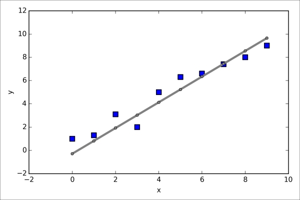
Let's start by creating a small one-dimensional toy dataset with five training samples:
>>> X_train = np.asarray([[0.0], [1.0], ... [2.0], [3.0], ... [4.0], [5.0], ... [6.0], [7.0], ... [8.0], [9.0]], ... dtype=theano.config.floatX) >>> y_train = np.asarray([1.0, 1.3, ... 3.1, 2.0, ... 5.0, 6.3, ... 6.6, 7.4, ... 8.0, 9.0], ... dtype=theano.config.floatX)
Note that we are using theano.config.floatX when we construct the NumPy arrays, so we can optionally toggle back and forth between CPU and GPU if we want.
Next, let's implement a training function to learn the weights of the linear regression model, using the sum of squared errors cost function. Note that is the bias unit (the y axis intercept at  ). The code is as follows:
import theano
from theano import tensor as T
import numpy as np
def train_linreg(X_train, y_train, eta, epochs):
costs = []
# Initialize arrays
eta0 = T.fscalar('eta0')
y = T.fvector(name='y')
X = T.fmatrix(name='X')
w = theano.shared(np.zeros(
shape=(X_train.shape[1] + 1),
dtype=theano.config.floatX),
name='w')
# calculate cost
net_input = T.dot(X, w[1:]) + w[0]
errors = y - net_input
cost = T.sum(T.pow(errors, 2))
# perform gradient update
gradient = T.grad(cost, wrt=w)
update = [(w, w - eta0 * gradient)]
# compile model
train = theano.function(inputs=[eta0],
outputs=cost,
updates=update,
givens={X: X_train,
y: y_train,})
for _ in range(epochs):
costs.append(train(eta))
return costs, wA really nice feature in Theano is the grad function that we used in the preceding code example. The grad function automatically computes the derivative of an expression with respect to its parameters that we passed to the function as the wrt argument.
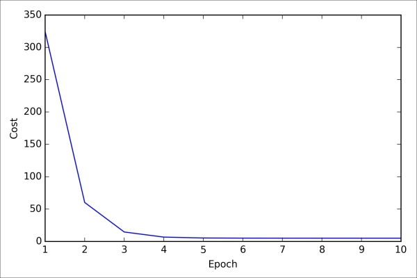
After we implemented the training function, let's train our linear regression model and take a look at the values of the Sum of Squared Errors (SSE) cost function to check if it converged:
>>> import matplotlib.pyplot as plt
>>> costs, w = train_linreg(X_train, y_train, eta=0.001, epochs=10)
>>> plt.plot(range(1, len(costs)+1), costs)
>>> plt.tight_layout()
>>> plt.xlabel('Epoch')
>>> plt.ylabel('Cost')
>>> plt.show()As we can see in the following plot, the learning algorithm already converged after the fifth epoch:
So far so good; by looking at the cost function, it seems that we built a working regression model from this particular dataset. Now, let's compile a new function to make predictions based on the input features:
def predict_linreg(X, w):
Xt = T.matrix(name='X')
net_input = T.dot(Xt, w[1:]) + w[0]
predict = theano.function(inputs=[Xt],
givens={w: w},
outputs=net_input)
return predict(X)Implementing a predict function was pretty straightforward following the three-step procedure of Theano: define, compile, and execute. Next, let's plot the linear regression fit on the training data:
>>> plt.scatter(X_train,
... y_train,
... marker='s',
... s=50)
>>> plt.plot(range(X_train.shape[0]),
... predict_linreg(X_train, w),
... color='gray',
... marker='o',
... markersize=4,
... linewidth=3)
>>> plt.xlabel('x')
>>> plt.ylabel('y')
>>> plt.show()As we can see in the resulting plot, our model fits the data points appropriately:
Implementing a simple regression model was a good exercise to become familiar with the Theano API. However, our ultimate goal is to play out the advantages of Theano, that is, implementing powerful artificial neural networks. We should now be equipped with all the tools we would need to implement the multilayer perceptron from Chapter 12, Training Artificial Neural Networks for Image Recognition, in Theano. However, this would be rather boring, right? Thus, we will take a look at one of my favorite deep learning libraries built on top of Theano to make the experimentation with neural networks as convenient as possible. However, before we introduce the Keras library, let's first discuss the different choices of activation functions in neural networks in the next section.
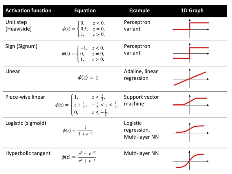
For simplicity, we have only discussed the sigmoid activation function in context of multilayer feedforward neural networks so far; we used in the hidden layer as well as the output layer in the multilayer perceptron implementation in Chapter 12, Training Artificial Neural Networks for Image Recognition. Although we referred to this activation function as sigmoid function—as it is commonly called in literature—the more precise definition would be logistic function or negative log-likelihood function. In the following subsections, you will learn more about alternative sigmoidal functions that are useful for implementing multilayer neural networks.
Technically, we could use any function as activation function in multilayer neural networks as long as it is differentiable. We could even use linear activation functions such as in Adaline (Chapter 2, Training Machine Learning Algorithms for Classification). However, in practice, it would not be very useful to use linear activation functions for both hidden and output layers, since we want to introduce nonlinearity in a typical artificial neural network to be able to tackle complex problem tasks. The sum of linear functions yields a linear function after all.
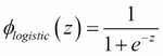
The logistic activation function that we used in the previous chapter probably mimics the concept of a neuron in a brain most closely: we can think of it as probability of whether a neuron fires or not. However, logistic activation functions can be problematic if we have highly negative inputs, since the output of the sigmoid function would be close to zero in this case. If the sigmoid function returns outputs that are close to zero, the neural network would learn very slowly and it becomes more likely that it gets trapped in local minima during training. This is why people often prefer a hyperbolic tangent as activation function in hidden layers. Before we discuss what a hyperbolic tangent looks like, let's briefly recapitulate some of the basics of the logistic function and look at a generalization that makes it more useful for multi-class classification tasks.
As we mentioned it in the introduction to this section, the logistic function, often just called the sigmoid function, is in fact a special case of a sigmoid function. We recall from the section on logistic regression in Chapter 3, A Tour of Machine Learning Classifiers Using Scikit-learn, that we can use the logistic function to model the probability that sample belongs to the positive class (class 1) in a binary classification task:
Here, the scalar variable is defined as the net input:
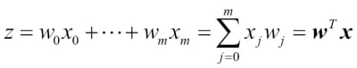
Note that is the bias unit (y-axis intercept,  ). To provide a more concrete example, let's assume a model for a two-dimensional data point x and a model with the following weight coefficients assigned to the vector
  :
:
>>> X = np.array([[1, 1.4, 1.5]])
>>> w = np.array([0.0, 0.2, 0.4])
>>> def net_input(X, w):
... z = X.dot(w)
... return z
>>> def logistic(z):
... return 1.0 / (1.0 + np.exp(-z))
>>> def logistic_activation(X, w):
... z = net_input(X, w)
... return logistic(z)
>>> print('P(y=1|x) = %.3f'
... % logistic_activation(X, w)[0])
P(y=1|x) = 0.707If we calculate the net input and use it to activate a logistic neuron with those particular feature values and weight coefficients, we get back a value of 0.707, which we can interpret as a 70.7 percent probability that this particular sample belongs to the positive class. In Chapter 12, Training Artificial Neural Networks for Image Recognition, we used the one-hot encoding technique to compute the values in the output layer consisting of multiple logistic activation units. However, as we will demonstrate with the following code example, an output layer consisting of multiple logistic activation units does not produce meaningful, interpretable probability values:
# W : array, shape = [n_output_units, n_hidden_units+1]
# Weight matrix for hidden layer -> output layer.
# note that first column (A[:][0] = 1) are the bias units
>>> W = np.array([[1.1, 1.2, 1.3, 0.5],
... [0.1, 0.2, 0.4, 0.1],
... [0.2, 0.5, 2.1, 1.9]])
# A : array, shape = [n_hidden+1, n_samples]
# Activation of hidden layer.
# note that first element (A[0][0] = 1) is the bias unit
>>> A = np.array([[1.0],
... [0.1],
... [0.3],
... [0.7]])
# Z : array, shape = [n_output_units, n_samples]
# Net input of the output layer.
>>> Z = W.dot(A)
>>> y_probas = logistic(Z)
>>> print('Probabilities:\n', y_probas)
Probabilities:
[[ 0.87653295]
[ 0.57688526]
[ 0.90114393]]As we can see in the output, the probability that the particular sample belongs to the first class is almost 88 percent, the probability that the particular sample belongs to the second class is almost 58 percent, and the probability that the particular sample belongs to the third class is 90 percent, respectively. This is clearly confusing, since we all know that a percentage should intuitively be expressed as a fraction of 100. However, this is in fact not a big concern if we only use our model to predict the class labels, not the class membership probabilities.
>>> y_class = np.argmax(Z, axis=0)
>>> print('predicted class label: %d' % y_class[0])
predicted class label: 2However, in certain contexts, it can be useful to return meaningful class probabilities for multi-class predictions. In the next section, we will take a look at a generalization of the logistic function, the softmax function, which can help us with this task.
The
softmax function is a generalization of the logistic function that allows us to compute meaningful class-probabilities in multi-class settings (multinomial logistic regression). In softmax, the probability of a particular sample with net input belongs to the  th class can be computed with a normalization term in the denominator that is the sum of all
  linear functions:
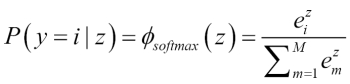
To see softmax in action, let's code it up in Python:
>>> def softmax(z):
... return np.exp(z) / np.sum(np.exp(z))
>>> def softmax_activation(X, w):
... z = net_input(X, w)
... return sigmoid(z)
>>> y_probas = softmax(Z)
>>> print('Probabilities:\n', y_probas)
Probabilities:
[[ 0.40386493]
[ 0.07756222]
[ 0.51857284]]
>>> y_probas.sum()
1.0As we can see, the predicted class probabilities now sum up to one, as we would expect. It is also notable that the probability for the second class is close to zero, since there is a large gap between  and
and  . However, note that the predicted class label is the same as in the logistic function. Intuitively, it may help to think of the softmax function as a normalized logistic function that is useful to obtain meaningful class-membership predictions in multi-class settings.
>>> y_class = np.argmax(Z, axis=0)
>>> print('predicted class label:
... %d' % y_class[0])
predicted class label: 2Another sigmoid function that is often used in the hidden layers of artificial neural networks is the hyperbolic tangent (tanh), which can be interpreted as a rescaled version of the logistic function.
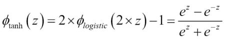

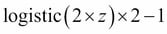
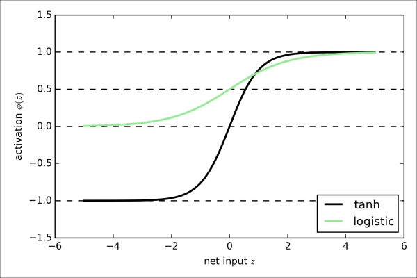
The advantage of the hyperbolic tangent over the logistic function is that it has a broader output spectrum and ranges the open interval (-1, 1), which can improve the convergence of the back propagation algorithm (C. M. Bishop. Neural networks for pattern recognition. Oxford university press, 1995, pp. 500-501). In contrast, the logistic function returns an output signal that ranges the open interval (0, 1). For an intuitive comparison of the logistic function and the hyperbolic tangent, let's plot two sigmoid functions in a one-dimensional space:
>>> import matplotlib.pyplot as plt
>>> def tanh(z):
... e_p = np.exp(z)
... e_m = np.exp(-z)
... return (e_p - e_m) / (e_p + e_m)
>>> z = np.arange(-5, 5, 0.005)
>>> log_act = logistic(z)
>>> tanh_act = tanh(z)
>>> plt.ylim([-1.5, 1.5])
>>> plt.xlabel('net input $z$')
>>> plt.ylabel('activation $\phi(z)$')
>>> plt.axhline(1, color='black', linestyle='--')
>>> plt.axhline(0.5, color='black', linestyle='--')
>>> plt.axhline(0, color='black', linestyle='--')
>>> plt.axhline(-1, color='black', linestyle='--')
>>> plt.plot(z, tanh_act,
... linewidth=2,
... color='black',
... label='tanh')
>>> plt.plot(z, log_act,
... linewidth=2,
... color='lightgreen',
... label='logistic')
>>> plt.legend(loc='lower right')
>>> plt.tight_layout()
>>> plt.show()As we can see, the shapes of the two sigmoidal curves look very similar; however, the tanh function has 2x larger output space than the logistic function:
Note that we implemented the logistic and tanh functions verbosely for the purpose of illustration. In practice, we can use NumPy's tanh function to achieve the same results:
>>> tanh_act = np.tanh(z)
In addition, the logistic function is available in SciPy's special module:
>>> from scipy.special import expit >>> log_act = expit(z)
Now that we know more about the different activation functions that are commonly used in artificial neural networks, let's conclude this section with an overview of the different activation function that we encountered in this book.
Logistic function recap
As we mentioned it in the introduction to this section, the logistic function, often just called the sigmoid function, is in fact a special case of a sigmoid function. We recall from the section on logistic regression in Chapter 3, A Tour of Machine Learning Classifiers Using Scikit-learn, that we can use the logistic function to model the probability that sample belongs to the positive class (class 1) in a binary classification task:
Here, the scalar variable is defined as the net input:
Note that is the bias unit (y-axis intercept, ). To provide a more concrete example, let's assume a model for a two-dimensional data point x and a model with the following weight coefficients assigned to the vector :
>>> X = np.array([[1, 1.4, 1.5]])
>>> w = np.array([0.0, 0.2, 0.4])
>>> def net_input(X, w):
... z = X.dot(w)
... return z
>>> def logistic(z):
... return 1.0 / (1.0 + np.exp(-z))
>>> def logistic_activation(X, w):
... z = net_input(X, w)
... return logistic(z)
>>> print('P(y=1|x) = %.3f'
... % logistic_activation(X, w)[0])
P(y=1|x) = 0.707If we calculate the net input and use it to activate a logistic neuron with those particular feature values and weight coefficients, we get back a value of 0.707, which we can interpret as a 70.7 percent probability that this particular sample belongs to the positive class. In Chapter 12, Training Artificial Neural Networks for Image Recognition, we used the one-hot encoding technique to compute the values in the output layer consisting of multiple logistic activation units. However, as we will demonstrate with the following code example, an output layer consisting of multiple logistic activation units does not produce meaningful, interpretable probability values:
# W : array, shape = [n_output_units, n_hidden_units+1]
# Weight matrix for hidden layer -> output layer.
# note that first column (A[:][0] = 1) are the bias units
>>> W = np.array([[1.1, 1.2, 1.3, 0.5],
... [0.1, 0.2, 0.4, 0.1],
... [0.2, 0.5, 2.1, 1.9]])
# A : array, shape = [n_hidden+1, n_samples]
# Activation of hidden layer.
# note that first element (A[0][0] = 1) is the bias unit
>>> A = np.array([[1.0],
... [0.1],
... [0.3],
... [0.7]])
# Z : array, shape = [n_output_units, n_samples]
# Net input of the output layer.
>>> Z = W.dot(A)
>>> y_probas = logistic(Z)
>>> print('Probabilities:\n', y_probas)
Probabilities:
[[ 0.87653295]
[ 0.57688526]
[ 0.90114393]]As we can see in the output, the probability that the particular sample belongs to the first class is almost 88 percent, the probability that the particular sample belongs to the second class is almost 58 percent, and the probability that the particular sample belongs to the third class is 90 percent, respectively. This is clearly confusing, since we all know that a percentage should intuitively be expressed as a fraction of 100. However, this is in fact not a big concern if we only use our model to predict the class labels, not the class membership probabilities.
>>> y_class = np.argmax(Z, axis=0)
>>> print('predicted class label: %d' % y_class[0])
predicted class label: 2However, in certain contexts, it can be useful to return meaningful class probabilities for multi-class predictions. In the next section, we will take a look at a generalization of the logistic function, the softmax function, which can help us with this task.
The
softmax function is a generalization of the logistic function that allows us to compute meaningful class-probabilities in multi-class settings (multinomial logistic regression). In softmax, the probability of a particular sample with net input belongs to the th class can be computed with a normalization term in the denominator that is the sum of all linear functions:
To see softmax in action, let's code it up in Python:
>>> def softmax(z):
... return np.exp(z) / np.sum(np.exp(z))
>>> def softmax_activation(X, w):
... z = net_input(X, w)
... return sigmoid(z)
>>> y_probas = softmax(Z)
>>> print('Probabilities:\n', y_probas)
Probabilities:
[[ 0.40386493]
[ 0.07756222]
[ 0.51857284]]
>>> y_probas.sum()
1.0As we can see, the predicted class probabilities now sum up to one, as we would expect. It is also notable that the probability for the second class is close to zero, since there is a large gap between and . However, note that the predicted class label is the same as in the logistic function. Intuitively, it may help to think of the softmax function as a normalized logistic function that is useful to obtain meaningful class-membership predictions in multi-class settings.
>>> y_class = np.argmax(Z, axis=0)
>>> print('predicted class label:
... %d' % y_class[0])
predicted class label: 2Another sigmoid function that is often used in the hidden layers of artificial neural networks is the hyperbolic tangent (tanh), which can be interpreted as a rescaled version of the logistic function.
The advantage of the hyperbolic tangent over the logistic function is that it has a broader output spectrum and ranges the open interval (-1, 1), which can improve the convergence of the back propagation algorithm (C. M. Bishop. Neural networks for pattern recognition. Oxford university press, 1995, pp. 500-501). In contrast, the logistic function returns an output signal that ranges the open interval (0, 1). For an intuitive comparison of the logistic function and the hyperbolic tangent, let's plot two sigmoid functions in a one-dimensional space:
>>> import matplotlib.pyplot as plt
>>> def tanh(z):
... e_p = np.exp(z)
... e_m = np.exp(-z)
... return (e_p - e_m) / (e_p + e_m)
>>> z = np.arange(-5, 5, 0.005)
>>> log_act = logistic(z)
>>> tanh_act = tanh(z)
>>> plt.ylim([-1.5, 1.5])
>>> plt.xlabel('net input $z$')
>>> plt.ylabel('activation $\phi(z)$')
>>> plt.axhline(1, color='black', linestyle='--')
>>> plt.axhline(0.5, color='black', linestyle='--')
>>> plt.axhline(0, color='black', linestyle='--')
>>> plt.axhline(-1, color='black', linestyle='--')
>>> plt.plot(z, tanh_act,
... linewidth=2,
... color='black',
... label='tanh')
>>> plt.plot(z, log_act,
... linewidth=2,
... color='lightgreen',
... label='logistic')
>>> plt.legend(loc='lower right')
>>> plt.tight_layout()
>>> plt.show()As we can see, the shapes of the two sigmoidal curves look very similar; however, the tanh function has 2x larger output space than the logistic function:
Note that we implemented the logistic and tanh functions verbosely for the purpose of illustration. In practice, we can use NumPy's tanh function to achieve the same results:
>>> tanh_act = np.tanh(z)
In addition, the logistic function is available in SciPy's special module:
>>> from scipy.special import expit >>> log_act = expit(z)
Now that we know more about the different activation functions that are commonly used in artificial neural networks, let's conclude this section with an overview of the different activation function that we encountered in this book.
Estimating probabilities in multi-class classification via the softmax function
The
softmax function is a generalization of the logistic function that allows us to compute meaningful class-probabilities in multi-class settings (multinomial logistic regression). In softmax, the probability of a particular sample with net input belongs to the th class can be computed with a normalization term in the denominator that is the sum of all linear functions:
To see softmax in action, let's code it up in Python:
>>> def softmax(z):
... return np.exp(z) / np.sum(np.exp(z))
>>> def softmax_activation(X, w):
... z = net_input(X, w)
... return sigmoid(z)
>>> y_probas = softmax(Z)
>>> print('Probabilities:\n', y_probas)
Probabilities:
[[ 0.40386493]
[ 0.07756222]
[ 0.51857284]]
>>> y_probas.sum()
1.0As we can see, the predicted class probabilities now sum up to one, as we would expect. It is also notable that the probability for the second class is close to zero, since there is a large gap between and . However, note that the predicted class label is the same as in the logistic function. Intuitively, it may help to think of the softmax function as a normalized logistic function that is useful to obtain meaningful class-membership predictions in multi-class settings.
>>> y_class = np.argmax(Z, axis=0)
>>> print('predicted class label:
... %d' % y_class[0])
predicted class label: 2Another sigmoid function that is often used in the hidden layers of artificial neural networks is the hyperbolic tangent (tanh), which can be interpreted as a rescaled version of the logistic function.
The advantage of the hyperbolic tangent over the logistic function is that it has a broader output spectrum and ranges the open interval (-1, 1), which can improve the convergence of the back propagation algorithm (C. M. Bishop. Neural networks for pattern recognition. Oxford university press, 1995, pp. 500-501). In contrast, the logistic function returns an output signal that ranges the open interval (0, 1). For an intuitive comparison of the logistic function and the hyperbolic tangent, let's plot two sigmoid functions in a one-dimensional space:
>>> import matplotlib.pyplot as plt
>>> def tanh(z):
... e_p = np.exp(z)
... e_m = np.exp(-z)
... return (e_p - e_m) / (e_p + e_m)
>>> z = np.arange(-5, 5, 0.005)
>>> log_act = logistic(z)
>>> tanh_act = tanh(z)
>>> plt.ylim([-1.5, 1.5])
>>> plt.xlabel('net input $z$')
>>> plt.ylabel('activation $\phi(z)$')
>>> plt.axhline(1, color='black', linestyle='--')
>>> plt.axhline(0.5, color='black', linestyle='--')
>>> plt.axhline(0, color='black', linestyle='--')
>>> plt.axhline(-1, color='black', linestyle='--')
>>> plt.plot(z, tanh_act,
... linewidth=2,
... color='black',
... label='tanh')
>>> plt.plot(z, log_act,
... linewidth=2,
... color='lightgreen',
... label='logistic')
>>> plt.legend(loc='lower right')
>>> plt.tight_layout()
>>> plt.show()As we can see, the shapes of the two sigmoidal curves look very similar; however, the tanh function has 2x larger output space than the logistic function:
Note that we implemented the logistic and tanh functions verbosely for the purpose of illustration. In practice, we can use NumPy's tanh function to achieve the same results:
>>> tanh_act = np.tanh(z)
In addition, the logistic function is available in SciPy's special module:
>>> from scipy.special import expit >>> log_act = expit(z)
Now that we know more about the different activation functions that are commonly used in artificial neural networks, let's conclude this section with an overview of the different activation function that we encountered in this book.
Broadening the output spectrum by using a hyperbolic tangent
Another sigmoid function that is often used in the hidden layers of artificial neural networks is the hyperbolic tangent (tanh), which can be interpreted as a rescaled version of the logistic function.
The advantage of the hyperbolic tangent over the logistic function is that it has a broader output spectrum and ranges the open interval (-1, 1), which can improve the convergence of the back propagation algorithm (C. M. Bishop. Neural networks for pattern recognition. Oxford university press, 1995, pp. 500-501). In contrast, the logistic function returns an output signal that ranges the open interval (0, 1). For an intuitive comparison of the logistic function and the hyperbolic tangent, let's plot two sigmoid functions in a one-dimensional space:
>>> import matplotlib.pyplot as plt
>>> def tanh(z):
... e_p = np.exp(z)
... e_m = np.exp(-z)
... return (e_p - e_m) / (e_p + e_m)
>>> z = np.arange(-5, 5, 0.005)
>>> log_act = logistic(z)
>>> tanh_act = tanh(z)
>>> plt.ylim([-1.5, 1.5])
>>> plt.xlabel('net input $z$')
>>> plt.ylabel('activation $\phi(z)$')
>>> plt.axhline(1, color='black', linestyle='--')
>>> plt.axhline(0.5, color='black', linestyle='--')
>>> plt.axhline(0, color='black', linestyle='--')
>>> plt.axhline(-1, color='black', linestyle='--')
>>> plt.plot(z, tanh_act,
... linewidth=2,
... color='black',
... label='tanh')
>>> plt.plot(z, log_act,
... linewidth=2,
... color='lightgreen',
... label='logistic')
>>> plt.legend(loc='lower right')
>>> plt.tight_layout()
>>> plt.show()As we can see, the shapes of the two sigmoidal curves look very similar; however, the tanh function has 2x larger output space than the logistic function:
Note that we implemented the logistic and tanh functions verbosely for the purpose of illustration. In practice, we can use NumPy's tanh function to achieve the same results:
>>> tanh_act = np.tanh(z)
In addition, the logistic function is available in SciPy's special module:
>>> from scipy.special import expit >>> log_act = expit(z)
Now that we know more about the different activation functions that are commonly used in artificial neural networks, let's conclude this section with an overview of the different activation function that we encountered in this book.
In this section, we will take a look at Keras, one of the most recently developed libraries to facilitate neural network training. The development on Keras started in the early months of 2015; as of today, it has evolved into one of the most popular and widely used libraries that are built on top of Theano, and allows us to utilize our GPU to accelerate neural network training. One of its prominent features is that it's a very intuitive API, which allows us to implement neural networks in only a few lines of code. Once you have Theano installed, you can install Keras from PyPI by executing the following command from your terminal command line:
pip install Keras
For more information about Keras, please visit the official website at http://keras.io.
To see what neural network training via Keras looks like, let's implement a multilayer perceptron to classify the handwritten digits from the MNIST dataset, which we introduced in the previous chapter. The MNIST dataset can be downloaded from http://yann.lecun.com/exdb/mnist/ in four parts as listed here:
train-images-idx3-ubyte.gz: These are training set images (9912422 bytes)train-labels-idx1-ubyte.gz: These are training set labels (28881 bytes)t10k-images-idx3-ubyte.gz: These are test set images (1648877 bytes)t10k-labels-idx1-ubyte.gz: These are test set labels (4542 bytes)
After downloading and unzipped the archives, we place the files into a directory mnist in our current working directory, so that we can load the training as well as the test dataset using the following function:
import os
import struct
import numpy as np
def load_mnist(path, kind='train'):
"""Load MNIST data from `path`"""
labels_path = os.path.join(path,
'%s-labels-idx1-ubyte'
% kind)
images_path = os.path.join(path,
'%s-images-idx3-ubyte'
% kind)
with open(labels_path, 'rb') as lbpath:
magic, n = struct.unpack('>II',
lbpath.read(8))
labels = np.fromfile(lbpath,
dtype=np.uint8)
with open(images_path, 'rb') as imgpath:
magic, num, rows, cols = struct.unpack(">IIII",
imgpath.read(16))
images = np.fromfile(imgpath,
dtype=np.uint8).reshape(len(labels), 784)
return images, labels
X_train, y_train = load_mnist('mnist', kind='train')
print('Rows: %d, columns: %d' % (X_train.shape[0], X_train.shape[1]))
Rows: 60000, columns: 784
X_test, y_test = load_mnist('mnist', kind='t10k')
print('Rows: %d, columns: %d' % (X_test.shape[0], X_test.shape[1]))
Rows: 10000, columns: 784On the following pages, we will walk through the code examples for using Keras step by step, which you can directly execute from your Python interpreter. However, if you are interested in training the neural network on your GPU, you can either put it into a Python script, or download the respective code from the Packt Publishing website. In order to run the Python script on your GPU, execute the following command from the directory where the mnist_keras_mlp.py file is located:
THEANO_FLAGS=mode=FAST_RUN,device=gpu,floatX=float32 python mnist_keras_mlp.py
To continue with the preparation of the training data, let's cast the MNIST image array into 32-bit format:
>>> import theano >>> theano.config.floatX = 'float32' >>> X_train = X_train.astype(theano.config.floatX) >>> X_test = X_test.astype(theano.config.floatX)
Next, we need to convert the class labels (integers 0-9) into the one-hot format. Fortunately, Keras provides a convenient tool for this:
>>> from keras.utils import np_utils
>>> print('First 3 labels: ', y_train[:3])
First 3 labels: [5 0 4]
>>> y_train_ohe = np_utils.to_categorical(y_train)
>>> print('\nFirst 3 labels (one-hot):\n', y_train_ohe[:3])
First 3 labels (one-hot):
[[ 0. 0. 0. 0. 0. 1. 0. 0. 0. 0.]
[ 1. 0. 0. 0. 0. 0. 0. 0. 0. 0.]
[ 0. 0. 0. 0. 1. 0. 0. 0. 0. 0.]]Now, we can get to the interesting part and implement a neural network. Here, we will use the same architecture as in Chapter 12, Training Artificial Neural Networks for Image Recognition. However, we will replace the logistic units in the hidden layer with hyperbolic tangent activation functions, replace the logistic function in the output layer with softmax, and add an additional hidden layer. Keras makes these tasks very simple, as you can see in the following code implementation:
>>> from keras.models import Sequential >>> from keras.layers.core import Dense >>> from keras.optimizers import SGD >>> np.random.seed(1) >>> model = Sequential() >>> model.add(Dense(input_dim=X_train.shape[1], ... output_dim=50, ... init='uniform', ... activation='tanh')) >>> model.add(Dense(input_dim=50, ... output_dim=50, ... init='uniform', ... activation='tanh')) >>> model.add(Dense(input_dim=50, ... output_dim=y_train_ohe.shape[1], ... init='uniform', ... activation='softmax')) >>> sgd = SGD(lr=0.001, decay=1e-7, momentum=.9) >>> model.compile(loss='categorical_crossentropy', optimizer=sgd)
First, we initialize a new model using the Sequential class to implement a feedforward neural network. Then, we can add as many layers to it as we like. However, since the first layer that we add is the input layer, we have to make sure that the input_dim attribute matches the number of features (columns) in the training set (here, 768). Also, we have to make sure that the number of output units (output_dim) and input units (input_dim) of two consecutive layers match. In the preceding example, we added two hidden layers with 50 hidden units plus 1 bias unit each. Note that bias units are initialized to 0 in fully connected networks in Keras. This is in contrast to the MLP implementation in Chapter 12, Training Artificial Neural Networks for Image Recognition, where we initialized the bias units to 1, which is a more common (not necessarily better) convention.
Finally, the number of units in the output layer should be equal to the number of unique class labels—the number of columns in the one-hot encoded class label array. Before we can compile our model, we also have to define an optimizer. In the preceding example, we chose a stochastic gradient descent optimization, which we are already familiar with, from previous chapters. Furthermore, we can set values for the weight decay constant and momentum learning to adjust the learning rate at each epoch as discussed in Chapter 12, Training Artificial Neural Networks for Image Recognition. Lastly, we set the cost (or loss) function to categorical_crossentropy. The (binary) cross-entropy is just the technical term for the cost function in logistic regression, and the categorical cross-entropy is its generalization for multi-class predictions via softmax. After compiling the model, we can now train it by calling the fit method. Here, we are using mini-batch stochastic gradient with a batch size of 300 training samples per batch. We train the MLP over 50 epochs, and we can follow the optimization of the cost function during training by setting verbose=1. The validation_split parameter is especially handy, since it will reserve 10 percent of the training data (here, 6,000 samples) for validation after each epoch, so that we can check if the model is overfitting during training.
>>> model.fit(X_train, ... y_train_ohe, ... nb_epoch=50, ... batch_size=300, ... verbose=1, ... validation_split=0.1, ... show_accuracy=True) Train on 54000 samples, validate on 6000 samples Epoch 0 54000/54000 [==============================] - 1s - loss: 2.2290 - acc: 0.3592 - val_loss: 2.1094 - val_acc: 0.5342 Epoch 1 54000/54000 [==============================] - 1s - loss: 1.8850 - acc: 0.5279 - val_loss: 1.6098 - val_acc: 0.5617 Epoch 2 54000/54000 [==============================] - 1s - loss: 1.3903 - acc: 0.5884 - val_loss: 1.1666 - val_acc: 0.6707 Epoch 3 54000/54000 [==============================] - 1s - loss: 1.0592 - acc: 0.6936 - val_loss: 0.8961 - val_acc: 0.7615 […] Epoch 49 54000/54000 [==============================] - 1s - loss: 0.1907 - acc: 0.9432 - val_loss: 0.1749 - val_acc: 0.9482
Printing the value of the cost function is extremely useful during training, since we can quickly spot whether the cost is decreasing during training and stop the algorithm earlier if otherwise to tune the hyperparameters values.
To predict the class labels, we can then use the predict_classes method to return the class labels directly as integers:
>>> y_train_pred = model.predict_classes(X_train, verbose=0)
>>> print('First 3 predictions: ', y_train_pred[:3])
>>> First 3 predictions: [5 0 4]Finally, let's print the model accuracy on training and test sets:
>>> train_acc = np.sum(
... y_train == y_train_pred, axis=0) / X_train.shape[0]
>>> print('Training accuracy: %.2f%%' % (train_acc * 100))
Training accuracy: 94.51%
>>> y_test_pred = model.predict_classes(X_test, verbose=0)
>>> test_acc = np.sum(y_test == y_test_pred,
... axis=0) / X_test.shape[0]
print('Test accuracy: %.2f%%' % (test_acc * 100))
Test accuracy: 94.39%Note that this is just a very simple neural network without optimized tuning parameters. If you are interested in playing more with Keras, please feel free to further tweak the learning rate, momentum, weight decay, and number of hidden units.
Note
Although Keras is great library for implementing and experimenting with neural networks, there are many other Theano wrapper libraries that are worth mentioning. A prominent example is Pylearn2 (http://deeplearning.net/software/pylearn2/), which has been developed in the LISA lab in Montreal. Also, Lasagne (https://github.com/Lasagne/Lasagne) may be of interest to you if you prefer a more minimalistic but extensible library, that offers more control over the underlying Theano code.
I hope you enjoyed this last chapter of an exciting tour of machine learning. Throughout this book, we covered all of the essential topics that this field has to offer, and you should now be well equipped to put those techniques into action to solve real-world problems.
We started our journey with a brief overview of the different types of learning tasks: supervised learning, reinforcement learning, and unsupervised learning. We discussed several different learning algorithms that can be used for classification, starting with simple single-layer neural networks in Chapter 2, Training Machine Learning Algorithms for Classification. Then, we discussed more advanced classification algorithms in Chapter 3, A Tour of Machine Learning Classifiers Using Scikit-learn, and you learned about the most important aspects of a machine learning pipeline in Chapter 4, Building Good Training Sets – Data Preprocessing and Chapter 5, Compressing Data via Dimensionality Reduction. Remember that even the most advanced algorithm is limited by the information in the training data that it gets to learn from. In Chapter 6, Learning Best Practices for Model Evaluation and Hyperparameter Tuning, you learned about the best practices to build and evaluate predictive models, which is another important aspect in machine learning applications. If one single learning algorithm does not achieve the performance we desire, it can sometimes be helpful to create an ensemble of experts to make a prediction. We discussed this in Chapter 7, Combining Different Models for Ensemble Learning. In Chapter 8, Applying Machine Learning to Sentiment Analysis, we applied machine learning to analyze the probably most interesting form of data in the modern age that is dominated by social media platforms on the Internet: text documents. However, machine learning techniques are not limited to offline data analysis, and in Chapter 9, Embedding a Machine Learning Model into a Web Application, we saw how to embed a machine learning model into a web application to share it with the outside world. For the most part, our focus was on algorithms for classification, probably the most popular application of machine learning. However, this is not where it ends! In Chapter 10, Predicting Continuous Target Variables with Regression Analysis, we explored several algorithms for regression analysis to predict continuous-valued output values. Another exciting subfield of machine learning is clustering analysis, which can help us to find hidden structures in data even if our training data does not come with the right answers to learn from. We discussed this in Chapter 11, Working with Unlabeled Data – Clustering Analysis.
In the last two chapters of this book, we caught a glimpse of the most beautiful and most exciting algorithms in the whole machine learning field: artificial neural networks. Although deep learning really is beyond the scope of this book, I hope I could at least kindle your interest to follow the most recent advancement in this field. If you are considering a career as machine learning researcher, or even if you just want to keep up to date with the current advancement in this field, I can recommend you to follow the works of the leading experts in this field, such as Geoff Hinton (http://www.cs.toronto.edu/~hinton/), Andrew Ng (http://www.andrewng.org), Yann LeCun (http://yann.lecun.com), Juergen Schmidhuber (http://people.idsia.ch/~juergen/), and Yoshua Bengio (http://www.iro.umontreal.ca/~bengioy), just to name a few. Also, please do not hesitate to join the scikit-learn, Theano, and Keras mailing lists to participate in interesting discussions around these libraries, and machine learning in general. I am looking forward to meet you there! You are always welcome to contact me if you have any questions about this book or need some general tips about machine learning.
I hope this journey through the different aspects of machine learning was really worthwhile, and you learned many new and useful skills to advance your career and apply them to real-world problem solving.