
In the previous chapter, we focused on the best practices for tuning and evaluating different models for classification. In this chapter, we will build upon these techniques and explore different methods for constructing a set of classifiers that can often have a better predictive performance than any of its individual members. You will learn how to:
- Make predictions based on majority voting
- Reduce overfitting by drawing random combinations of the training set with repetition
- Build powerful models from weak learners that learn from their mistakes
The goal behind ensemble methods is to combine different classifiers into a meta-classifier that has a better generalization performance than each individual classifier alone. For example, assuming that we collected predictions from 10 experts, ensemble methods would allow us to strategically combine these predictions by the 10 experts to come up with a prediction that is more accurate and robust than the predictions by each individual expert. As we will see later in this chapter, there are several different approaches for creating an ensemble of classifiers. In this section, we will introduce a basic perception about how ensembles work and why they are typically recognized for yielding a good generalization performance.
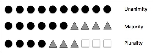
In this chapter, we will focus on the most popular ensemble methods that use the majority voting principle. Majority voting simply means that we select the class label that has been predicted by the majority of classifiers, that is, received more than 50 percent of the votes. Strictly speaking, the term majority vote refers to binary class settings only. However, it is easy to generalize the majority voting principle to multi-class settings, which is called plurality voting. Here, we select the class label that received the most votes (mode). The following diagram illustrates the concept of majority and plurality voting for an ensemble of 10 classifiers where each unique symbol (triangle, square, and circle) represents a unique class label:
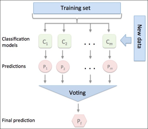
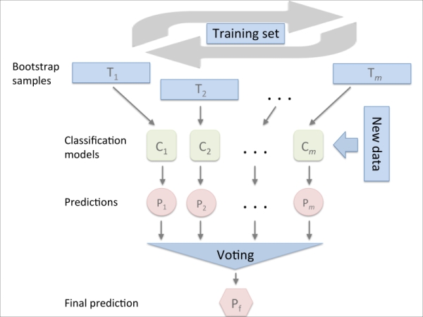
Using the training set, we start by training m different classifiers ( ). Depending on the technique, the ensemble can be built from different classification algorithms, for example, decision trees, support vector machines, logistic regression classifiers, and so on. Alternatively, we can also use the same base classification algorithm fitting different subsets of the training set. One prominent example of this approach would be the random forest algorithm, which combines different decision tree classifiers. The following diagram illustrates the concept of a general ensemble approach using majority voting:
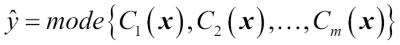
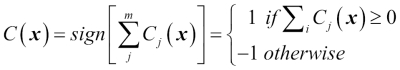
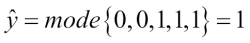
To predict a class label via a simple majority or plurality voting, we combine the predicted class labels of each individual classifier  and select the class label
  that received the most votes:
For example, in a binary classification task where  and
and  , we can write the majority vote prediction as follows:
To illustrate why ensemble methods can work better than individual classifiers alone, let's apply the simple concepts of combinatorics. For the following example, we make the assumption that all n base classifiers for a binary classification task have an equal error rate  . Furthermore, we assume that the classifiers are independent and the error rates are not correlated. Under those assumptions, we can simply express the error probability of an ensemble of base classifiers as a probability mass function of a binomial distribution:
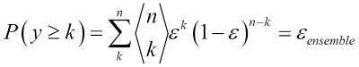
Here,  is the binomial coefficient n choose k. In other words, we compute the probability that the prediction of the ensemble is wrong. Now let's take a look at a more concrete example of 11 base classifiers (
 ) with an error rate of 0.25 (
 ):
):
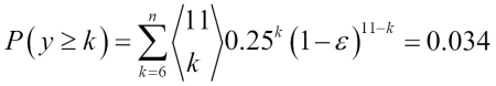
As we can see, the error rate of the ensemble (0.034) is much lower than the error rate of each individual classifier (0.25) if all the assumptions are met. Note that, in this simplified illustration, a 50-50 split by an even number of classifiers n is treated as an error, whereas this is only true half of the time. To compare such an idealistic ensemble classifier to a base classifier over a range of different base error rates, let's implement the probability mass function in Python:
>>> from scipy.misc import comb >>> import math >>> def ensemble_error(n_classifier, error): ... k_start = math.ceil(n_classifier / 2.0) ... probs = [comb(n_classifier, k) * ... error**k * ... (1-error)**(n_classifier - k) ... for k in range(k_start, n_classifier + 1)] ... return sum(probs) >>> ensemble_error(n_classifier=11, error=0.25) 0.034327507019042969
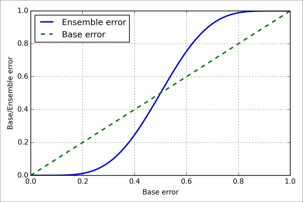
After we've implemented the ensemble_error function, we can compute the ensemble error rates for a range of different base errors from 0.0 to 1.0 to visualize the relationship between ensemble and base errors in a line graph:
>>> import numpy as np
>>> error_range = np.arange(0.0, 1.01, 0.01)
>>> ens_errors = [ensemble_error(n_classifier=11, error=error)
... for error in error_range]
>>> import matplotlib.pyplot as plt
>>> plt.plot(error_range, ens_errors,
... label='Ensemble error',
... linewidth=2)
>>> plt.plot(error_range, error_range,
... linestyle='--', label='Base error',
... linewidth=2)
>>> plt.xlabel('Base error')
>>> plt.ylabel('Base/Ensemble error')
>>> plt.legend(loc='upper left')
>>> plt.grid()
>>> plt.show()As we can see in the resulting plot, the error probability of an ensemble is always better than the error of an individual base classifier as long as the base classifiers perform better than random guessing ( ). Note that the y-axis depicts the base error (dotted line) as well as the ensemble error (continuous line):
After the short introduction to ensemble learning in the previous section, let's start with a warm-up exercise and implement a simple ensemble classifier for majority voting in Python. Although the following algorithm also generalizes to multi-class settings via plurality voting, we will use the term majority voting for simplicity as is also often done in literature.
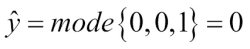
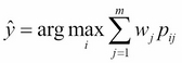
The algorithm that we are going to implement will allow us to combine different classification algorithms associated with individual weights for confidence. Our goal is to build a stronger meta-classifier that balances out the individual classifiers' weaknesses on a particular dataset. In more precise mathematical terms, we can write the weighted majority vote as follows:

Here,  is a weight associated with a base classifier, ,
  is the predicted class label of the ensemble,
  (Greek chi) is the characteristic function
  , and A is the set of unique class labels. For equal weights, we can simplify this equation and write it as follows:

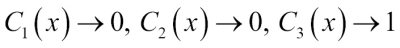
To better understand the concept of weighting, we will now take a look at a more concrete example. Let's assume that we have an ensemble of three base classifiers ( and want to predict the class label of a given sample instance x. Two out of three base classifiers predict the class label 0, and one
  predicts that the sample belongs to class 1. If we weight the predictions of each base classifier equally, the majority vote will predict that the sample belongs to class 0:
Now let's assign a weight of 0.6 to and weight  and
and  by a coefficient of 0.2, respectively.
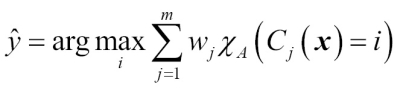
More intuitively, since  , we can say that the prediction made by has three times more weight than the predictions by or , respectively. We can write this as follows:
To translate the concept of the weighted majority vote into Python code, we can use NumPy's convenient argmax and bincount functions:
>>> import numpy as np >>> np.argmax(np.bincount([0, 0, 1], ... weights=[0.2, 0.2, 0.6])) 1
As discussed in Chapter 3, A Tour of Machine Learning Classifiers Using Scikit-learn, certain classifiers in scikit-learn can also return the probability of a predicted class label via the predict_proba method. Using the predicted class probabilities instead of the class labels for majority voting can be useful if the classifiers in our ensemble are well calibrated. The modified version of the majority vote for predicting class labels from probabilities can be written as follows:
Here,  is the predicted probability of the jth classifier for class label i.
To continue with our previous example, let's assume that we have a binary classification problem with class labels  and an ensemble of three classifiers
  (
( ). Let's assume that the classifier returns the following class membership probabilities for a particular sample
  :
:

We can then calculate the individual class probabilities as follows:


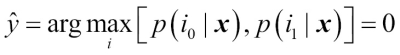
To implement the weighted majority vote based on class probabilities, we can again make use of NumPy using numpy.average and np.argmax:
>>> ex = np.array([[0.9, 0.1], ... [0.8, 0.2], ... [0.4, 0.6]]) >>> p = np.average(ex, axis=0, weights=[0.2, 0.2, 0.6]) >>> p array([ 0.58, 0.42]) >>> np.argmax(p) 0
Putting everything together, let's now implement a MajorityVoteClassifier in Python:
from sklearn.base import BaseEstimator
from sklearn.base import ClassifierMixin
from sklearn.preprocessing import LabelEncoder
from sklearn.externals import six
from sklearn.base import clone
from sklearn.pipeline import _name_estimators
import numpy as np
import operator
class MajorityVoteClassifier(BaseEstimator,
ClassifierMixin):
""" A majority vote ensemble classifier
Parameters
----------
classifiers : array-like, shape = [n_classifiers]
Different classifiers for the ensemble
vote : str, {'classlabel', 'probability'}
Default: 'classlabel'
If 'classlabel' the prediction is based on
the argmax of class labels. Else if
'probability', the argmax of the sum of
probabilities is used to predict the class label
(recommended for calibrated classifiers).
weights : array-like, shape = [n_classifiers]
Optional, default: None
If a list of `int` or `float` values are
provided, the classifiers are weighted by
importance; Uses uniform weights if `weights=None`.
"""
def __init__(self, classifiers,
vote='classlabel', weights=None):
self.classifiers = classifiers
self.named_classifiers = {key: value for
key, value in
_name_estimators(classifiers)}
self.vote = vote
self.weights = weights
def fit(self, X, y):
""" Fit classifiers.
Parameters
----------
X : {array-like, sparse matrix},
shape = [n_samples, n_features]
Matrix of training samples.
y : array-like, shape = [n_samples]
Vector of target class labels.
Returns
-------
self : object
"""
# Use LabelEncoder to ensure class labels start
# with 0, which is important for np.argmax
# call in self.predict
self.lablenc_ = LabelEncoder()
self.lablenc_.fit(y)
self.classes_ = self.lablenc_.classes_
self.classifiers_ = []
for clf in self.classifiers:
fitted_clf = clone(clf).fit(X,
self.lablenc_.transform(y))
self.classifiers_.append(fitted_clf)
return selfI added a lot of comments to the code to better understand the individual parts. However, before we implement the remaining methods, let's take a quick break and discuss some of the code that may look confusing at first. We used the parent classes BaseEstimator and ClassifierMixin to get some base functionality for free, including the methods get_params and set_params to set and return the classifier's parameters as well as the score method to calculate the prediction accuracy, respectively. Also note that we imported six to make the MajorityVoteClassifier compatible with Python 2.7.
Next we will add the predict method to predict the class label via majority vote based on the class labels if we initialize a new MajorityVoteClassifier object with vote='classlabel'. Alternatively, we will be able to initialize the ensemble classifier with vote='probability' to predict the class label based on the class membership probabilities. Furthermore, we will also add a predict_proba method to return the average probabilities, which is useful to compute the Receiver Operator Characteristic area under the curve (ROC AUC).
def predict(self, X):
""" Predict class labels for X.
Parameters
----------
X : {array-like, sparse matrix},
Shape = [n_samples, n_features]
Matrix of training samples.
Returns
----------
maj_vote : array-like, shape = [n_samples]
Predicted class labels.
"""
if self.vote == 'probability':
maj_vote = np.argmax(self.predict_proba(X),
axis=1)
else: # 'classlabel' vote
# Collect results from clf.predict calls
predictions = np.asarray([clf.predict(X)
for clf in
self.classifiers_]).T
maj_vote = np.apply_along_axis(
lambda x:
np.argmax(np.bincount(x,
weights=self.weights)),
axis=1,
arr=predictions)
maj_vote = self.lablenc_.inverse_transform(maj_vote)
return maj_vote
def predict_proba(self, X):
""" Predict class probabilities for X.
Parameters
----------
X : {array-like, sparse matrix},
shape = [n_samples, n_features]
Training vectors, where n_samples is
the number of samples and
n_features is the number of features.
Returns
----------
avg_proba : array-like,
shape = [n_samples, n_classes]
Weighted average probability for
each class per sample.
"""
probas = np.asarray([clf.predict_proba(X)
for clf in self.classifiers_])
avg_proba = np.average(probas,
axis=0, weights=self.weights)
return avg_proba
def get_params(self, deep=True):
""" Get classifier parameter names for GridSearch"""
if not deep:
return super(MajorityVoteClassifier,
self).get_params(deep=False)
else:
out = self.named_classifiers.copy()
for name, step in\
six.iteritems(self.named_classifiers):
for key, value in six.iteritems(
step.get_params(deep=True)):
out['%s__%s' % (name, key)] = value
return outAlso, note that we defined our own modified version of the get_params methods to use the _name_estimators function in order to access the parameters of individual classifiers in the ensemble. This may look a little bit complicated at first, but it will make perfect sense when we use grid search for hyperparameter-tuning in later sections.
Now it is about time to put the MajorityVoteClassifier that we implemented in the previous section into action. But first, let's prepare a dataset that we can test it on. Since we are already familiar with techniques to load datasets from CSV files, we will take a shortcut and load the Iris dataset from scikit-learn's dataset module. Furthermore, we will only select two features, sepal width and
petal length, to make the classification task more challenging. Although our MajorityVoteClassifier generalizes to multiclass problems, we will only classify flower samples from the two classes, Iris-Versicolor and Iris-Virginica, to compute the
ROC AUC. The code is as follows:
>>> from sklearn import datasets >>> from sklearn.cross_validation import train_test_split >>> from sklearn.preprocessing import StandardScaler >>> from sklearn.preprocessing import LabelEncoder >>> iris = datasets.load_iris() >>> X, y = iris.data[50:, [1, 2]], iris.target[50:] >>> le = LabelEncoder() >>> y = le.fit_transform(y)
Note
Note that scikit-learn uses the predict_proba method (if applicable) to compute the ROC AUC score. In Chapter 3, A Tour of Machine Learning Classifiers Using Scikit-learn, we saw how the class probabilities are computed in logistic regression models. In decision trees, the probabilities are calculated from a frequency vector that is created for each node at training time. The vector collects the frequency values of each class label computed from the class label distribution at that node. Then the frequencies are normalized so that they sum up to 1. Similarly, the class labels of the k-nearest neighbors are aggregated to return the normalized class label frequencies in the k-nearest neighbors algorithm. Although the normalized probabilities returned by both the decision tree and k-nearest neighbors classifier may look similar to the probabilities obtained from a logistic regression model, we have to be aware that these are actually not derived from probability mass functions.
Next we split the Iris samples into 50 percent training and 50 percent test data:
>>> X_train, X_test, y_train, y_test =\ ... train_test_split(X, y, ... test_size=0.5, ... random_state=1)
Using the training dataset, we now will train three different classifiers—a logistic regression classifier, a decision tree classifier, and a k-nearest neighbors classifier—and look at their individual performances via a 10-fold cross-validation on the training dataset before we combine them into an ensemble classifier:
>>> from sklearn.cross_validation import cross_val_score
>>> from sklearn.linear_model import LogisticRegression
>>> from sklearn.tree import DecisionTreeClassifier
>>> from sklearn.neighbors import KNeighborsClassifier
>>> from sklearn.pipeline import Pipeline
>>> import numpy as np
>>> clf1 = LogisticRegression(penalty='l2',
... C=0.001,
... random_state=0)
>>> clf2 = DecisionTreeClassifier(max_depth=1,
... criterion='entropy',
... random_state=0)
>>> clf3 = KNeighborsClassifier(n_neighbors=1,
... p=2,
... metric='minkowski')
>>> pipe1 = Pipeline([['sc', StandardScaler()],
... ['clf', clf1]])
>>> pipe3 = Pipeline([['sc', StandardScaler()],
... ['clf', clf3]])
>>> clf_labels = ['Logistic Regression', 'Decision Tree', 'KNN']
>>> print('10-fold cross validation:\n')
>>> for clf, label in zip([pipe1, clf2, pipe3], clf_labels):
... scores = cross_val_score(estimator=clf,
>>> X=X_train,
>>> y=y_train,
>>> cv=10,
>>> scoring='roc_auc')
>>> print("ROC AUC: %0.2f (+/- %0.2f) [%s]"
... % (scores.mean(), scores.std(), label))The output that we receive, as shown in the following snippet, shows that the predictive performances of the individual classifiers are almost equal:
10-fold cross validation: ROC AUC: 0.92 (+/- 0.20) [Logistic Regression] ROC AUC: 0.92 (+/- 0.15) [Decision Tree] ROC AUC: 0.93 (+/- 0.10) [KNN]
You may be wondering why we trained the logistic regression and k-nearest neighbors classifier as part of a pipeline. The reason behind it is that, as discussed in Chapter 3, A Tour of Machine Learning Classifiers Using Scikit-learn, both the logistic regression and k-nearest neighbors algorithms (using the Euclidean distance metric) are not scale-invariant in contrast with decision trees. Although the Iris features are all measured on the same scale (cm), it is a good habit to work with standardized features.
Now let's move on to the more exciting part and combine the individual classifiers for majority rule voting in our MajorityVoteClassifier:
>>> mv_clf = MajorityVoteClassifier(
... classifiers=[pipe1, clf2, pipe3])
>>> clf_labels += ['Majority Voting']
>>> all_clf = [pipe1, clf2, pipe3, mv_clf]
>>> for clf, label in zip(all_clf, clf_labels):
... scores = cross_val_score(estimator=clf,
... X=X_train,
... y=y_train,
... cv=10,
... scoring='roc_auc')
... print("Accuracy: %0.2f (+/- %0.2f) [%s]"
... % (scores.mean(), scores.std(), label))
ROC AUC: 0.92 (+/- 0.20) [Logistic Regression]
ROC AUC: 0.92 (+/- 0.15) [Decision Tree]
ROC AUC: 0.93 (+/- 0.10) [KNN]
ROC AUC: 0.97 (+/- 0.10) [Majority Voting]As we can see, the performance of the MajorityVotingClassifier has substantially improved over the individual classifiers in the 10-fold cross-validation evaluation.
Combining different algorithms for classification with majority vote
Now it is about time to put the MajorityVoteClassifier that we implemented in the previous section into action. But first, let's prepare a dataset that we can test it on. Since we are already familiar with techniques to load datasets from CSV files, we will take a shortcut and load the Iris dataset from scikit-learn's dataset module. Furthermore, we will only select two features, sepal width and
petal length, to make the classification task more challenging. Although our MajorityVoteClassifier generalizes to multiclass problems, we will only classify flower samples from the two classes, Iris-Versicolor and Iris-Virginica, to compute the
ROC AUC. The code is as follows:
>>> from sklearn import datasets >>> from sklearn.cross_validation import train_test_split >>> from sklearn.preprocessing import StandardScaler >>> from sklearn.preprocessing import LabelEncoder >>> iris = datasets.load_iris() >>> X, y = iris.data[50:, [1, 2]], iris.target[50:] >>> le = LabelEncoder() >>> y = le.fit_transform(y)
Note
Note that scikit-learn uses the predict_proba method (if applicable) to compute the ROC AUC score. In Chapter 3, A Tour of Machine Learning Classifiers Using Scikit-learn, we saw how the class probabilities are computed in logistic regression models. In decision trees, the probabilities are calculated from a frequency vector that is created for each node at training time. The vector collects the frequency values of each class label computed from the class label distribution at that node. Then the frequencies are normalized so that they sum up to 1. Similarly, the class labels of the k-nearest neighbors are aggregated to return the normalized class label frequencies in the k-nearest neighbors algorithm. Although the normalized probabilities returned by both the decision tree and k-nearest neighbors classifier may look similar to the probabilities obtained from a logistic regression model, we have to be aware that these are actually not derived from probability mass functions.
Next we split the Iris samples into 50 percent training and 50 percent test data:
>>> X_train, X_test, y_train, y_test =\ ... train_test_split(X, y, ... test_size=0.5, ... random_state=1)
Using the training dataset, we now will train three different classifiers—a logistic regression classifier, a decision tree classifier, and a k-nearest neighbors classifier—and look at their individual performances via a 10-fold cross-validation on the training dataset before we combine them into an ensemble classifier:
>>> from sklearn.cross_validation import cross_val_score
>>> from sklearn.linear_model import LogisticRegression
>>> from sklearn.tree import DecisionTreeClassifier
>>> from sklearn.neighbors import KNeighborsClassifier
>>> from sklearn.pipeline import Pipeline
>>> import numpy as np
>>> clf1 = LogisticRegression(penalty='l2',
... C=0.001,
... random_state=0)
>>> clf2 = DecisionTreeClassifier(max_depth=1,
... criterion='entropy',
... random_state=0)
>>> clf3 = KNeighborsClassifier(n_neighbors=1,
... p=2,
... metric='minkowski')
>>> pipe1 = Pipeline([['sc', StandardScaler()],
... ['clf', clf1]])
>>> pipe3 = Pipeline([['sc', StandardScaler()],
... ['clf', clf3]])
>>> clf_labels = ['Logistic Regression', 'Decision Tree', 'KNN']
>>> print('10-fold cross validation:\n')
>>> for clf, label in zip([pipe1, clf2, pipe3], clf_labels):
... scores = cross_val_score(estimator=clf,
>>> X=X_train,
>>> y=y_train,
>>> cv=10,
>>> scoring='roc_auc')
>>> print("ROC AUC: %0.2f (+/- %0.2f) [%s]"
... % (scores.mean(), scores.std(), label))The output that we receive, as shown in the following snippet, shows that the predictive performances of the individual classifiers are almost equal:
10-fold cross validation: ROC AUC: 0.92 (+/- 0.20) [Logistic Regression] ROC AUC: 0.92 (+/- 0.15) [Decision Tree] ROC AUC: 0.93 (+/- 0.10) [KNN]
You may be wondering why we trained the logistic regression and k-nearest neighbors classifier as part of a pipeline. The reason behind it is that, as discussed in Chapter 3, A Tour of Machine Learning Classifiers Using Scikit-learn, both the logistic regression and k-nearest neighbors algorithms (using the Euclidean distance metric) are not scale-invariant in contrast with decision trees. Although the Iris features are all measured on the same scale (cm), it is a good habit to work with standardized features.
Now let's move on to the more exciting part and combine the individual classifiers for majority rule voting in our MajorityVoteClassifier:
>>> mv_clf = MajorityVoteClassifier(
... classifiers=[pipe1, clf2, pipe3])
>>> clf_labels += ['Majority Voting']
>>> all_clf = [pipe1, clf2, pipe3, mv_clf]
>>> for clf, label in zip(all_clf, clf_labels):
... scores = cross_val_score(estimator=clf,
... X=X_train,
... y=y_train,
... cv=10,
... scoring='roc_auc')
... print("Accuracy: %0.2f (+/- %0.2f) [%s]"
... % (scores.mean(), scores.std(), label))
ROC AUC: 0.92 (+/- 0.20) [Logistic Regression]
ROC AUC: 0.92 (+/- 0.15) [Decision Tree]
ROC AUC: 0.93 (+/- 0.10) [KNN]
ROC AUC: 0.97 (+/- 0.10) [Majority Voting]As we can see, the performance of the MajorityVotingClassifier has substantially improved over the individual classifiers in the 10-fold cross-validation evaluation.
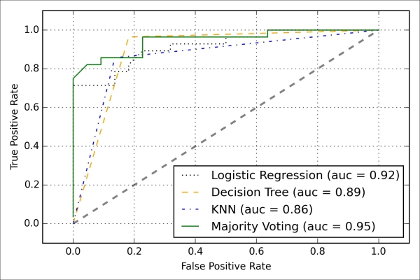
In this section, we are going to compute the ROC curves from the test set to check if the MajorityVoteClassifier generalizes well to unseen data. We should remember that the test set is not to be used for model selection; its only purpose is to report an unbiased estimate of the generalization performance of a classifier system. The code is as follows:
>>> from sklearn.metrics import roc_curve
>>> from sklearn.metrics import auc
>>> colors = ['black', 'orange', 'blue', 'green']
>>> linestyles = [':', '--', '-.', '-']
>>> for clf, label, clr, ls \
... in zip(all_clf, clf_labels, colors, linestyles):
... # assuming the label of the positive class is 1
... y_pred = clf.fit(X_train,
... y_train).predict_proba(X_test)[:, 1]
... fpr, tpr, thresholds = roc_curve(y_true=y_test,
... y_score=y_pred)
... roc_auc = auc(x=fpr, y=tpr)
... plt.plot(fpr, tpr,
... color=clr,
... linestyle=ls,
... label='%s (auc = %0.2f)' % (label, roc_auc))
>>> plt.legend(loc='lower right')
>>> plt.plot([0, 1], [0, 1],
... linestyle='--',
... color='gray',
... linewidth=2)
>>> plt.xlim([-0.1, 1.1])
>>> plt.ylim([-0.1, 1.1])
>>> plt.grid()
>>> plt.xlabel('False Positive Rate')
>>> plt.ylabel('True Positive Rate')
>>> plt.show()As we can see in the resulting ROC, the ensemble classifier also performs well on the test set (ROC AUC = 0.95), whereas the k-nearest neighbors classifier seems to be overfitting the training data (training ROC AUC = 0.93, test ROC AUC = 0.86):
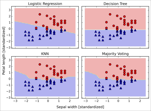
Since we only selected two features for the classification examples, it would be interesting to see what the decision region of the ensemble classifier actually looks like. Although it is not necessary to standardize the training features prior to model fitting because our logistic regression and k-nearest neighbors pipelines will automatically take care of this, we will standardize the training set so that the decision regions of the decision tree will be on the same scale for visual purposes. The code is as follows:
>>> sc = StandardScaler() >>> X_train_std = sc.fit_transform(X_train) >>> from itertools import product >>> x_min = X_train_std[:, 0].min() - 1 >>> x_max = X_train_std[:, 0].max() + 1 >>> y_min = X_train_std[:, 1].min() - 1 >>> y_max = X_train_std[:, 1].max() + 1 >>> xx, yy = np.meshgrid(np.arange(x_min, x_max, 0.1), ... np.arange(y_min, y_max, 0.1)) >>> f, axarr = plt.subplots(nrows=2, ncols=2, ... sharex='col', ... sharey='row', ... figsize=(7, 5)) >>> for idx, clf, tt in zip(product([0, 1], [0, 1]), ... all_clf, clf_labels): ... clf.fit(X_train_std, y_train) ... Z = clf.predict(np.c_[xx.ravel(), yy.ravel()]) ... Z = Z.reshape(xx.shape) ... axarr[idx[0], idx[1]].contourf(xx, yy, Z, alpha=0.3) ... axarr[idx[0], idx[1]].scatter(X_train_std[y_train==0, 0], ... X_train_std[y_train==0, 1], ... c='blue', ... marker='^', ... s=50) ... axarr[idx[0], idx[1]].scatter(X_train_std[y_train==1, 0], ... X_train_std[y_train==1, 1], ... c='red', ... marker='o', ... s=50) ... axarr[idx[0], idx[1]].set_title(tt) >>> plt.text(-3.5, -4.5, ... s='Sepal width [standardized]', ... ha='center', va='center', fontsize=12) >>> plt.text(-10.5, 4.5, ... s='Petal length [standardized]', ... ha='center', va='center', ... fontsize=12, rotation=90) >>> plt.show()
Interestingly but also as expected, the decision regions of the ensemble classifier seem to be a hybrid of the decision regions from the individual classifiers. At first glance, the majority vote decision boundary looks a lot like the decision boundary of the k-nearest neighbor classifier. However, we can see that it is orthogonal to the y axis for  , just like the decision tree stump:
Before you learn how to tune the individual classifier parameters for ensemble classification, let's call the get_params method to get a basic idea of how we can access the individual parameters inside a GridSearch object:
>>> mv_clf.get_params()
{'decisiontreeclassifier': DecisionTreeClassifier(class_weight=None, criterion='entropy', max_depth=1,
max_features=None, max_leaf_nodes=None, min_samples_leaf=1,
min_samples_split=2, min_weight_fraction_leaf=0.0,
random_state=0, splitter='best'),
'decisiontreeclassifier__class_weight': None,
'decisiontreeclassifier__criterion': 'entropy',
[...]
'decisiontreeclassifier__random_state': 0,
'decisiontreeclassifier__splitter': 'best',
'pipeline-1': Pipeline(steps=[('sc', StandardScaler(copy=True, with_mean=True, with_std=True)), ('clf', LogisticRegression(C=0.001, class_weight=None, dual=False, fit_intercept=True,
intercept_scaling=1, max_iter=100, multi_class='ovr',
penalty='l2', random_state=0, solver='liblinear', tol=0.0001,
verbose=0))]),
'pipeline-1__clf': LogisticRegression(C=0.001, class_weight=None, dual=False, fit_intercept=True,
intercept_scaling=1, max_iter=100, multi_class='ovr',
penalty='l2', random_state=0, solver='liblinear', tol=0.0001,
verbose=0),
'pipeline-1__clf__C': 0.001,
'pipeline-1__clf__class_weight': None,
'pipeline-1__clf__dual': False,
[...]
'pipeline-1__sc__with_std': True,
'pipeline-2': Pipeline(steps=[('sc', StandardScaler(copy=True, with_mean=True, with_std=True)), ('clf', KNeighborsClassifier(algorithm='auto', leaf_size=30, metric='minkowski',
metric_params=None, n_neighbors=1, p=2, weights='uniform'))]),
'pipeline-2__clf': KNeighborsClassifier(algorithm='auto', leaf_size=30, metric='minkowski',
metric_params=None, n_neighbors=1, p=2, weights='uniform'),
'pipeline-2__clf__algorithm': 'auto',
[...]
'pipeline-2__sc__with_std': True}Based on the values returned by the get_params method, we now know how to access the individual classifier's attributes. Let's now tune the inverse regularization parameter C of the logistic regression classifier and the decision tree depth via a grid search for demonstration purposes. The code is as follows:
>>> from sklearn.grid_search import GridSearchCV
>>> params = {'decisiontreeclassifier__max_depth': [1, 2],
... 'pipeline-1__clf__C': [0.001, 0.1, 100.0]}
>>> grid = GridSearchCV(estimator=mv_clf,
... param_grid=params,
... cv=10,
... scoring='roc_auc')
>>> grid.fit(X_train, y_train)After the grid search has completed, we can print the different hyperparameter value combinations and the average ROC AUC scores computed via 10-fold cross-validation. The code is as follows:
>>> for params, mean_score, scores in grid.grid_scores_:
... print("%0.3f+/-%0.2f %r"
... % (mean_score, scores.std() / 2, params))
0.967+/-0.05 {'pipeline-1__clf__C': 0.001, 'decisiontreeclassifier__max_depth': 1}
0.967+/-0.05 {'pipeline-1__clf__C': 0.1, 'decisiontreeclassifier__max_depth': 1}
1.000+/-0.00 {'pipeline-1__clf__C': 100.0, 'decisiontreeclassifier__max_depth': 1}
0.967+/-0.05 {'pipeline-1__clf__C': 0.001, 'decisiontreeclassifier__max_depth': 2}
0.967+/-0.05 {'pipeline-1__clf__C': 0.1, 'decisiontreeclassifier__max_depth': 2}
1.000+/-0.00 {'pipeline-1__clf__C': 100.0, 'decisiontreeclassifier__max_depth': 2}
>>> print('Best parameters: %s' % grid.best_params_)
Best parameters: {'pipeline-1__clf__C': 100.0, 'decisiontreeclassifier__max_depth': 1}
>>> print('Accuracy: %.2f' % grid.best_score_)
Accuracy: 1.00As we can see, we get the best cross-validation results when we choose a lower regularization strength (C = 100.0) whereas the tree depth does not seem to affect the performance at all, suggesting that a decision stump is sufficient to separate the data. To remind ourselves that it is a bad practice to use the test dataset more than once for model evaluation, we are not going to estimate the generalization performance of the tuned hyperparameters in this section. We will move on swiftly to an alternative approach for ensemble learning: bagging.
Note
The majority vote approach we implemented in this section is sometimes also referred to as stacking. However, the stacking algorithm is more typically used in combination with a logistic regression model that predicts the final class label using the predictions of the individual classifiers in the ensemble as input, which has been described in more detail by David H. Wolpert in D. H. Wolpert. Stacked generalization. Neural networks, 5(2):241–259, 1992.
Bagging is an ensemble learning technique that is closely related to the MajorityVoteClassifier that we implemented in the previous section, as illustrated in the following diagram:
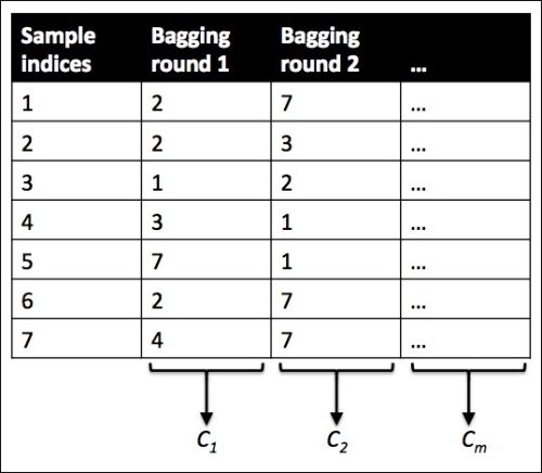
However, instead of using the same training set to fit the individual classifiers in the ensemble, we draw bootstrap samples (random samples with replacement) from the initial training set, which is why bagging is also known as
bootstrap aggregating. To provide a more concrete example of how bootstrapping works, let's consider the example shown in the following figure. Here, we have seven different training instances (denoted as indices 1-7) that are sampled randomly with replacement in each round of bagging. Each bootstrap sample is then used to fit a classifier , which is most typically an unpruned decision tree:
Bagging is also related to the random forest classifier that we introduced in Chapter 3, A Tour of Machine Learning Classifiers Using Scikit-learn. In fact, random forests are a special case of bagging where we also use random feature subsets to fit the individual decision trees. Bagging was first proposed by Leo Breiman in a technical report in 1994; he also showed that bagging can improve the accuracy of unstable models and decrease the degree of overfitting. I highly recommend you read about his research in L. Breiman. Bagging Predictors. Machine Learning, 24(2):123–140, 1996, which is freely available online, to learn more about bagging.
To see bagging in action, let's create a more complex classification problem using the Wine dataset that we introduced in Chapter 4, Building Good Training Sets – Data Preprocessing. Here, we will only consider the Wine classes 2 and 3, and we select two features: Alcohol and Hue.
>>> import pandas as pd
>>> df_wine = pd.read_csv('https://archive.ics.uci.edu/ml/machine-learning-databases/wine/wine.data', header=None)
>>> df_wine.columns = ['Class label', 'Alcohol',
... 'Malic acid', 'Ash',
... 'Alcalinity of ash',
... 'Magnesium', 'Total phenols',
... 'Flavanoids', 'Nonflavanoid phenols',
... 'Proanthocyanins',
... 'Color intensity', 'Hue',
... 'OD280/OD315 of diluted wines',
... 'Proline']
>>> df_wine = df_wine[df_wine['Class label'] != 1]
>>> y = df_wine['Class label'].values
>>> X = df_wine[['Alcohol', 'Hue']].valuesNext we encode the class labels into binary format and split the dataset into 60 percent training and 40 percent test set, respectively:
>>> from sklearn.preprocessing import LabelEncoder >>> from sklearn.cross_validation import train_test_split >>> le = LabelEncoder() >>> y = le.fit_transform(y) >>> X_train, X_test, y_train, y_test =\ ... train_test_split(X, y, ... test_size=0.40, ... random_state=1)
A BaggingClassifier algorithm is already implemented in scikit-learn, which we can import from the ensemble submodule. Here, we will use an unpruned decision tree as the base classifier and create an ensemble of 500 decision trees fitted on different bootstrap samples of the training dataset:
>>> from sklearn.ensemble import BaggingClassifier >>> tree = DecisionTreeClassifier(criterion='entropy', ... max_depth=None) >>> bag = BaggingClassifier(base_estimator=tree, ... n_estimators=500, ... max_samples=1.0, ... max_features=1.0, ... bootstrap=True, ... bootstrap_features=False, ... n_jobs=1, ... random_state=1)
Next we will calculate the accuracy score of the prediction on the training and test dataset to compare the performance of the bagging classifier to the performance of a single unpruned decision tree:
>>> from sklearn.metrics import accuracy_score
>>> tree = tree.fit(X_train, y_train)
>>> y_train_pred = tree.predict(X_train)
>>> y_test_pred = tree.predict(X_test)
>>> tree_train = accuracy_score(y_train, y_train_pred)
>>> tree_test = accuracy_score(y_test, y_test_pred)
>>> print('Decision tree train/test accuracies %.3f/%.3f'
... % (tree_train, tree_test))
Decision tree train/test accuracies 1.000/0.854Based on the accuracy values that we printed by executing the preceding code snippet, the unpruned decision tree predicts all class labels of the training samples correctly; however, the substantially lower test accuracy indicates high variance (overfitting) of the model:
>>> bag = bag.fit(X_train, y_train)
>>> y_train_pred = bag.predict(X_train)
>>> y_test_pred = bag.predict(X_test)
>>> bag_train = accuracy_score(y_train, y_train_pred)
>>> bag_test = accuracy_score(y_test, y_test_pred)
>>> print('Bagging train/test accuracies %.3f/%.3f'
... % (bag_train, bag_test))
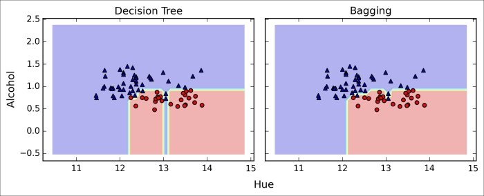
Bagging train/test accuracies 1.000/0.896Although the training accuracies of the decision tree and bagging classifier are similar on the training set (both 1.0), we can see that the bagging classifier has a slightly better generalization performance as estimated on the test set. Next let's compare the decision regions between the decision tree and bagging classifier:
>>> x_min = X_train[:, 0].min() - 1 >>> x_max = X_train[:, 0].max() + 1 >>> y_min = X_train[:, 1].min() - 1 >>> y_max = X_train[:, 1].max() + 1 >>> xx, yy = np.meshgrid(np.arange(x_min, x_max, 0.1), ... np.arange(y_min, y_max, 0.1)) >>> f, axarr = plt.subplots(nrows=1, ncols=2, ... sharex='col', ... sharey='row', ... figsize=(8, 3)) >>> for idx, clf, tt in zip([0, 1], ... [tree, bag], ... ['Decision Tree', 'Bagging']): ... clf.fit(X_train, y_train) ... ... Z = clf.predict(np.c_[xx.ravel(), yy.ravel()]) ... Z = Z.reshape(xx.shape) ... axarr[idx].contourf(xx, yy, Z, alpha=0.3) ... axarr[idx].scatter(X_train[y_train==0, 0], ... X_train[y_train==0, 1], ... c='blue', marker='^') ... axarr[idx].scatter(X_train[y_train==1, 0], ... X_train[y_train==1, 1], ... c='red', marker='o') ... axarr[idx].set_title(tt) >>> axarr[0].set_ylabel(Alcohol', fontsize=12) >>> plt.text(10.2, -1.2, ... s=Hue', ... ha='center', va='center', fontsize=12) >>> plt.show()
As we can see in the resulting plot, the piece-wise linear decision boundary of the three-node deep decision tree looks smoother in the bagging ensemble:
We only looked at a very simple bagging example in this section. In practice, more complex classification tasks and datasets' high dimensionality can easily lead to overfitting in single decision trees and this is where the bagging algorithm can really play out its strengths. Finally, we shall note that the bagging algorithm can be an effective approach to reduce the variance of a model. However, bagging is ineffective in reducing model bias, which is why we want to choose an ensemble of classifiers with low bias, for example, unpruned decision trees.
In this section about ensemble methods, we will discuss boosting with a special focus on its most common implementation, AdaBoost (short for Adaptive Boosting).
Note
The original idea behind AdaBoost was formulated by Robert Schapire in 1990 (R. E. Schapire. The Strength of Weak Learnability. Machine learning, 5(2):197–227, 1990). After Robert Schapire and Yoav Freund presented the AdaBoost algorithm in the Proceedings of the Thirteenth International Conference (ICML 1996), AdaBoost became one of the most widely used ensemble methods in the years that followed (Y. Freund, R. E. Schapire, et al. Experiments with a New Boosting Algorithm. In ICML, volume 96, pages 148–156, 1996). In 2003, Freund and Schapire received the Goedel Prize for their groundbreaking work, which is a prestigious prize for the most outstanding publications in the computer science field.
In boosting, the ensemble consists of very simple base classifiers, also often referred to as weak learners, that have only a slight performance advantage over random guessing. A typical example of a weak learner would be a decision tree stump. The key concept behind boosting is to focus on training samples that are hard to classify, that is, to let the weak learners subsequently learn from misclassified training samples to improve the performance of the ensemble. In contrast to bagging, the initial formulation of boosting, the algorithm uses random subsets of training samples drawn from the training dataset without replacement. The original boosting procedure is summarized in four key steps as follows:
-
Draw a random subset of training samples
 without replacement from the training set
  to train a weak learner .
-
Draw second random training subset
 without replacement from the training set and add 50 percent of the samples that were previously misclassified to train a weak learner .
-
Find the training samples
 in the training set on which and disagree to train a third weak learner .
-
Combine the weak learners , , and via majority voting.
As discussed by Leo Breiman (L. Breiman. Bias, Variance, and Arcing Classifiers. 1996), boosting can lead to a decrease in bias as well as variance compared to bagging models. In practice, however, boosting algorithms such as AdaBoost are also known for their high variance, that is, the tendency to overfit the training data (G. Raetsch, T. Onoda, and K. R. Mueller. An Improvement of Adaboost to Avoid Overfitting. In Proc. of the Int. Conf. on Neural Information Processing. Citeseer, 1998).
In contrast to the original boosting procedure as described here, AdaBoost uses the complete training set to train the weak learners where the training samples are reweighted in each iteration to build a strong classifier that learns from the mistakes of the previous weak learners in the ensemble. Before we dive deeper into the specific details of the AdaBoost algorithm, let's take a look at the following figure to get a better grasp of the basic concept behind AdaBoost:
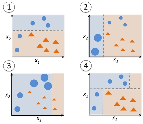
To walk through the AdaBoost illustration step by step, we start with subfigure 1, which represents a training set for binary classification where all training samples are assigned equal weights. Based on this training set, we train a decision stump (shown as a dashed line) that tries to classify the samples of the two classes (triangles and circles) as well as possible by minimizing the cost function (or the impurity score in the special case of decision tree ensembles). For the next round (subfigure 2), we assign a larger weight to the two previously misclassified samples (circles). Furthermore, we lower the weight of the correctly classified samples. The next decision stump will now be more focused on the training samples that have the largest weights, that is, the training samples that are supposedly hard to classify. The weak learner shown in subfigure 2 misclassifies three different samples from the circle-class, which are then assigned a larger weight as shown in subfigure 3. Assuming that our AdaBoost ensemble only consists of three rounds of boosting, we would then combine the three weak learners trained on different reweighted training subsets by a weighted majority vote, as shown in subfigure 4.
Now that have a better understanding behind the basic concept of AdaBoost, let's take a more detailed look at the algorithm using pseudo code. For clarity, we will denote element-wise multiplication by the cross symbol  and the dot product between two vectors by a dot symbol
  , respectively. The steps are as follows:
-
Set weight vector
 to uniform weights where
- For j in m boosting rounds, do the following:
-
Train a weighted weak learner:
 ).
).
-
Predict class labels:
 .
.
-
Compute weighted error rate:
 .
.
-
Compute coefficient:
 .
.
-
Update weights:
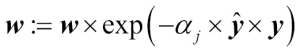 .
.
-
Normalize weights to sum to 1:
 .
.
-
Compute final prediction:
 .
.
Note that the expression  in step 5 refers to a vector of 1s and 0s, where a 1 is assigned if the prediction is correct and 0 is assigned otherwise.
Although the AdaBoost algorithm seems to be pretty straightforward, let's walk through a more concrete example using a training set consisting of 10 training samples as illustrated in the following table:
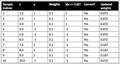
The first column of the table depicts the sample indices of the training samples 1 to 10. In the second column, we see the feature values of the individual samples assuming this is a one-dimensional dataset. The third column shows the true class label  for each training sample
  , where
  . The initial weights are shown in the fourth column; we initialize the weights to uniform and normalize them to sum to one. In the case of the 10 sample training set, we therefore assign the 0.1 to each weight
  in the weight vector . The predicted class labels
  are shown in the fifth column, assuming that our splitting criterion is
  . The last column of the table then shows the updated weights based on the update rules that we defined in the pseudocode.
Since the computation of the weight updates may look a little bit complicated at first, we will now follow the calculation step by step. We start by computing the weighted error rate as described in step 5:
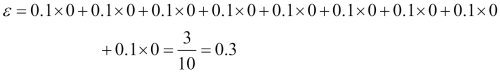
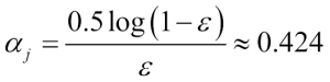
Next we compute the coefficient  (shown in step 6), which is later used in step 7 to update the weights as well as for the weights in majority vote prediction (step 10):
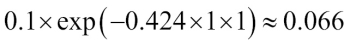
After we have computed the coefficient we can now update the weight vector using the following equation:
Here,  is an element-wise multiplication between the vectors of the predicted and true class labels, respectively. Thus, if a prediction
  is correct,
  will have a positive sign so that we decrease the ith weight since is a positive number as well:
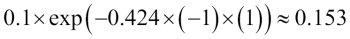
Similarly, we will downweight the ith weight if predicted the label incorrectly like this:
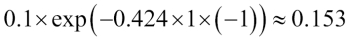
Or like this:
After we update each weight in the weight vector, we normalize the weights so that they sum up to 1 (step 8):

Here,  .
.
Thus, each weight that corresponds to a correctly classified sample will be reduced from the initial value of 0.1 to  for the next round of boosting. Similarly, the weights of each incorrectly classified sample will increase from 0.1 to
  .
.
This was AdaBoost in a nutshell. Skipping to the more practical part, let's now train an AdaBoost ensemble classifier via scikit-learn. We will use the same Wine subset that we used in the previous section to train the bagging meta-classifier. Via the base_estimator attribute, we will train the AdaBoostClassifier on 500 decision tree stumps:
>>> from sklearn.ensemble import AdaBoostClassifier
>>> tree = DecisionTreeClassifier(criterion='entropy',
... max_depth=1)
>>> ada = AdaBoostClassifier(base_estimator=tree,
... n_estimators=500,
... learning_rate=0.1,
... random_state=0)
>>> tree = tree.fit(X_train, y_train)
>>> y_train_pred = tree.predict(X_train)
>>> y_test_pred = tree.predict(X_test)
>>> tree_train = accuracy_score(y_train, y_train_pred)
>>> tree_test = accuracy_score(y_test, y_test_pred)
>>> print('Decision tree train/test accuracies %.3f/%.3f'
... % (tree_train, tree_test))
Decision tree train/test accuracies 0.845/0.854As we can see, the decision tree stump seems to overfit the training data in contrast with the unpruned decision tree that we saw in the previous section:
>>> ada = ada.fit(X_train, y_train)
>>> y_train_pred = ada.predict(X_train)
>>> y_test_pred = ada.predict(X_test)
>>> ada_train = accuracy_score(y_train, y_train_pred)
>>> ada_test = accuracy_score(y_test, y_test_pred)
>>> print('AdaBoost train/test accuracies %.3f/%.3f'
... % (ada_train, ada_test))
AdaBoost train/test accuracies 1.000/0.875As we can see, the AdaBoost model predicts all class labels of the training set correctly and also shows a slightly improved test set performance compared to the decision tree stump. However, we also see that we introduced additional variance by our attempt to reduce the model bias.
Although we used another simple example for demonstration purposes, we can see that the performance of the AdaBoost classifier is slightly improved compared to the decision stump and achieved very similar accuracy scores to the bagging classifier that we trained in the previous section. However, we should note that it is considered as bad practice to select a model based on the repeated usage of the test set. The estimate of the generalization performance may be too optimistic, which we discussed in more detail in Chapter 6, Learning Best Practices for Model Evaluation and Hyperparameter Tuning.
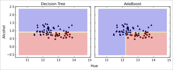
Finally, let's check what the decision regions look like:
>>> x_min = X_train[:, 0].min() - 1
>>> x_max = X_train[:, 0].max() + 1
>>> y_min = X_train[:, 1].min() - 1
>>> y_max = X_train[:, 1].max() + 1
>>> xx, yy = np.meshgrid(np.arange(x_min, x_max, 0.1),
... np.arange(y_min, y_max, 0.1))
>>> f, axarr = plt.subplots(1, 2,
... sharex='col',
... sharey='row',
... figsize=(8, 3))
>>> for idx, clf, tt in zip([0, 1],
... [tree, ada],
... ['Decision Tree', 'AdaBoost']):
... clf.fit(X_train, y_train)
... Z = clf.predict(np.c_[xx.ravel(), yy.ravel()])
... Z = Z.reshape(xx.shape)
... axarr[idx].contourf(xx, yy, Z, alpha=0.3)
... axarr[idx].scatter(X_train[y_train==0, 0],
... X_train[y_train==0, 1],
... c='blue',
... marker='^')
... axarr[idx].scatter(X_train[y_train==1, 0],
... X_train[y_train==1, 1],
... c='red',
... marker='o')
... axarr[idx].set_title(tt)
... axarr[0].set_ylabel('Alcohol', fontsize=12)
>>> plt.text(10.2, -1.2,
... s=Hue',
... ha='center',
... va='center',
... fontsize=12)
>>> plt.show()By looking at the decision regions, we can see that the decision boundary of the AdaBoost model is substantially more complex than the decision boundary of the decision stump. In addition, we note that the AdaBoost model separates the feature space very similarly to the bagging classifier that we trained in the previous section.
As concluding remarks about ensemble techniques, it is worth noting that ensemble learning increases the computational complexity compared to individual classifiers. In practice, we need to think carefully whether we want to pay the price of increased computational costs for an often relatively modest improvement of predictive performance.
An often-cited example of this trade-off is the famous $1 Million Netflix Prize, which was won using ensemble techniques. The details about the algorithm were published in A. Toescher, M. Jahrer, and R. M. Bell. The Bigchaos Solution to the Netflix Grand Prize. Netflix prize documentation, 2009 (which is available at http://www.stat.osu.edu/~dmsl/GrandPrize2009_BPC_BigChaos.pdf). Although the winning team received the $1 million prize money, Netflix never implemented their model due to its complexity, which made it unfeasible for a real-world application. To quote their exact words (http://techblog.netflix.com/2012/04/netflix-recommendations-beyond-5-stars.html):
"[…] additional accuracy gains that we measured did not seem to justify the engineering effort needed to bring them into a production environment."
In this chapter, we looked at some of the most popular and widely used techniques for ensemble learning. Ensemble methods combine different classification models to cancel out their individual weakness, which often results in stable and well-performing models that are very attractive for industrial applications as well as machine learning competitions.
In the beginning of this chapter, we implemented a MajorityVoteClassifier in Python that allows us to combine different algorithm for classification. We then looked at bagging, a useful technique to reduce the variance of a model by drawing random bootstrap samples from the training set and combining the individually trained classifiers via majority vote. Then we discussed AdaBoost, which is an algorithm that is based on weak learners that subsequently learn from mistakes.
Throughout the previous chapters, we discussed different learning algorithms, tuning, and evaluation techniques. In the following chapter, we will look at a particular application of machine learning, sentiment analysis, which has certainly become an interesting topic in the era of the Internet and social media.