The deep neural network architectures can vary greatly in structure depending on the network's application, but they all have some basic components. In this section, we will talk briefly about those components.

In this book, I'll define a deep neural network as a network with more than a single hidden layer. Beyond that we won't attempt to limit the membership to the Deep Learning Club. As such, our networks might have less than 100 neurons, or possibly millions. We might use special layers of neurons, including convolutions and recurrent layers, but we will refer to all of these as neurons nonetheless.

A neuron is the atomic unit of a neural network. This is sometimes inspired by biology; however, that's a topic for a different book. Neurons are typically arranged into layers. In this book, if I'm referring to a specific neuron, I'll use the notation where l is the layer the neuron is in and k is the neuron number. As we will be using programming languages that observe 0th notation, my notation will also be 0th based.

At their core, most neurons are composed of two functions that work together: a linear function and an activation function. Let us take a high-level look at those two components.

The first component of the neuron is a linear function whose output is the sum of the inputs, each multiplied by a coefficient. This function is really more or less a linear regression. These coefficients are typically referred to as weights in neural network speak. For example, given some neuron with the input features of x1, x2, and x3, and output z, this linear component or the neuron linear function would simply be:

Where are weights or coefficients that we will need to learn given the data and b is a bias term.

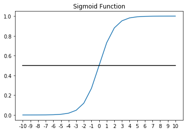
The second function of the neuron is the activation function, which is tasked with introducing a nonlinearity between neurons. A commonly used activation is the sigmoid activation, which you may be familiar with from logistic regression. It squeezes the output of the neuron into an output space where very large values of z are driven to 1 and very small values of z are driven to 0.

The sigmoid function looks like this:

It turns out that the activation function is very important for intermediate neurons. Without it one could prove that a stack of neurons with linear activation's (which is really no activation, or more formally an activation function where z=z) is really just a single linear function.

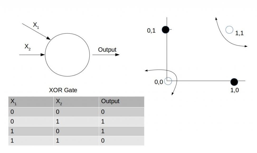
A single linear function is undesirable in this case because there are many scenarios where our network may be under specified for the problem at hand. That is to say that the network can't model the data well because of non-linear relationships present in the data between the input features and target variable (what we're predicting).

The canonical example of a function that cannot be modeled with a linear function is the exclusive OR function, which is shown in the following figure:

Other common activation functions are the tanh function and the ReLu or Rectilinear Activation.

The hyperbolic tangent or the tanh function looks like this:

>

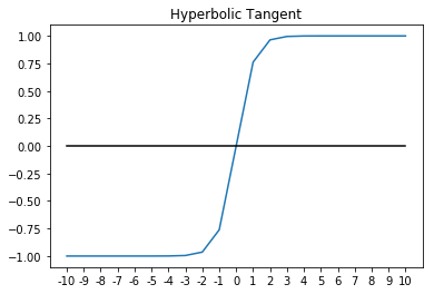
The tanh usually works better than sigmoid for intermediate layers. As you can probably see, the output of tanh will be between [-1, 1], whereas the output of sigmoid is [0, 1]. This additional width provides some resilience from a phenomenon known as the vanishing/exploding gradient problem, which we will cover in more detail later. For now, it's enough to know that the vanishing gradient problem can cause networks to converge very slowly in the early layers, if at all. Because of that, networks using tanh will tend to converge somewhat faster than networks that use sigmoid activation. That said, they are still not as fast as ReLu.

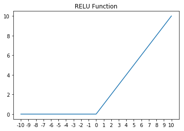
ReLu, or Rectilinear Activation, is defined simply as:

It's a safe bet and we will use it most of the time throughout this book. Not only is ReLu easy to compute and differentiate, it's also resilient against the vanishing gradient problem. The only drawback to ReLu is that it's first derivative is undefined at exactly 0. Variants including leaky ReLu, are computationally harder, but more robust against this issue.

For completeness, here's a somewhat obvious graph of ReLu:

Every machine learning model really starts with a cost function. Simply, a cost function allows you to measure how well your model is fitting the training data. In this book, we will define the loss function as the correctness of fit for a single observation within the training set. The cost function will then most often be an average of the loss across the training set. We will revisit loss functions later when we introduce each type of neural network; however, quickly consider the cost function for linear regression as an example:

In this case, the loss function would be , which is really the squared error. So then J, our cost function, is really just the mean squared error, or an average of the squared error across the entire dataset. The term 1/2 is added to make some of the calculus cleaner by convention.

Forward propagation is the process by which we attempt to predict our target variable using the features present in a single observation. Imagine we had a two-layer neural network. In the forward propagation process, we would start with the features present within that observation and then multiply those features by their associated coefficients within layer 1 and add a bias term for each neuron. After that, we would send that output to the activation for the neuron. Following that, the output would be sent to the next layer, and so on, until we reach the end of the network where we are left with our network's prediction:

>

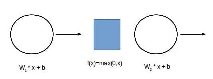
Once forward propagation is complete, we have the network's prediction for each data point. We also know that data point's actual value. Typically, the prediction is defined as while the actual value of the target variable is defined as y.

Once both y and are known, the network's error can be computed using the cost function. Recall that the cost function is the average of the loss function.

In order for learning to occur within the network, the network's error signal must be propagated backwards through the network layers from the last layer to the first. Our goal in back propagation is to propagate this error signal backwards through the network while using it to update the network weights as the signal travels. Mathematically, to do so we need to minimize the cost function by nudging the weights towards values that make the cost function the smallest. This process is called gradient descent.

The gradient is the partial derivative of the error function with respect to each weight within the network. The gradient of each weight can be calculated, layer by layer, using the chain rule and the gradients of the layers above.

Once the gradients of each layer are known, we can use the gradient descent algorithm to minimize the cost function.

The Gradient Descent will repeat this update until the network's error is minimized and the process has converged:

The gradient descent algorithm multiples the gradient by a learning rate called alpha and subtracts that value from the current value of each weight. The learning rate is a hyperparameter.

The algorithm describe in the previous section assumes a forward and corresponding backwards pass over the entire dataset and as such it's called batch gradient descent.

Another possible way to do gradient descent would be to use a single data point at a time, updating the network weights as we go. This method might help speed up convergence around saddle points where the network might stop converging. Of course, the error estimation of only a single point may not be a very good approximation of the error of the entire dataset.

The best solution to this problem is using mini batch gradient descent, in which we will take some random subset of the data called a mini batch to compute our error and update our network weights. This is almost always the best option. It has the additional benefit of naturally splitting a very large dataset into chunks that are more easily managed in the memory of a machine, or even across machines.