

Creating your first measure – where to go
Before we create our first measure, it would be a good idea to store all our measures in one table. This will make it easier to organize our measures and separate them from other fields in our data.
To create such a measures table, follow these steps:
- Select an empty cell in your worksheet.
- Copy the empty cell and click on the Manage button, as shown in the following screenshot:
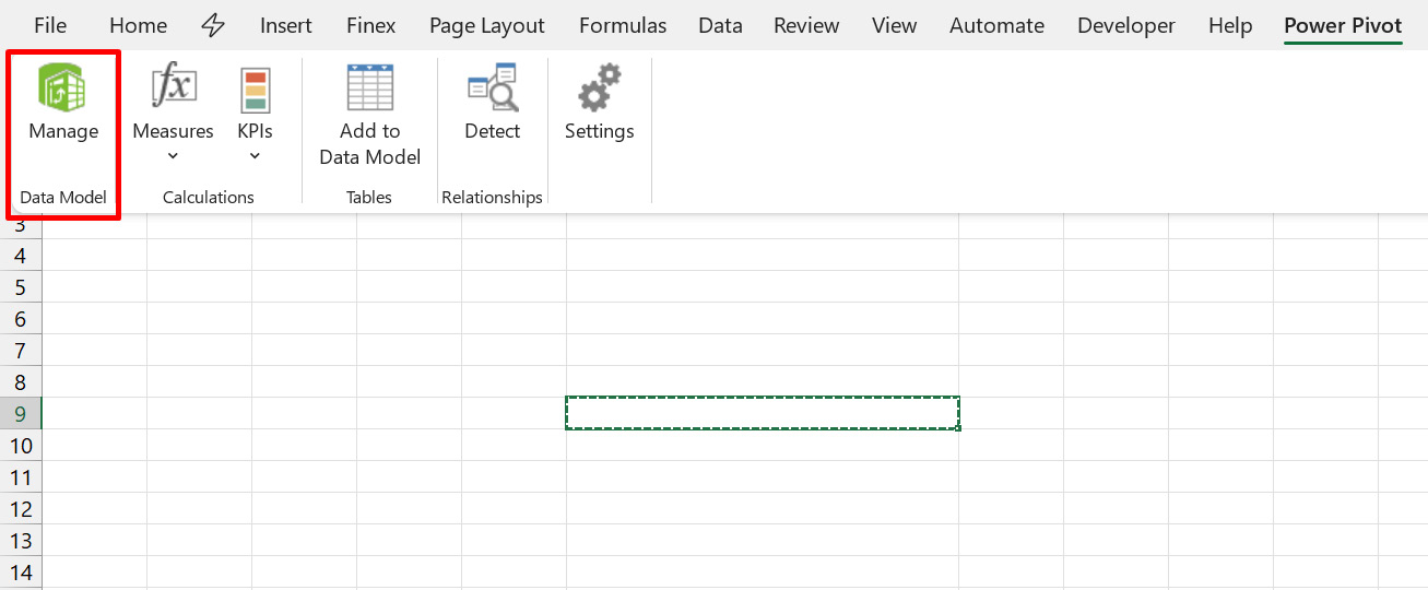
Figure 5.2 – Creating a table for measures
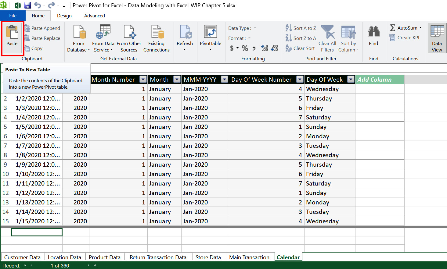
Figure 5.3 – The Paste dialog box in Power Pivot
This brings up the following Paste Preview dialog box:
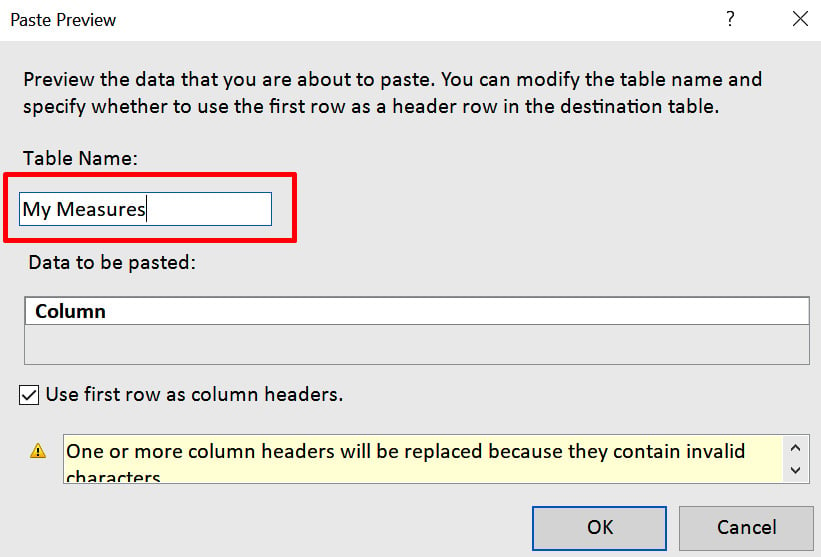
Figure 5.4 – Naming your measures
You can now assign a new name to the table. In my case, I named it My Measures. Click OK to finish the process.