Book Image

Applied Supervised Learning with R

By : Karthik Ramasubramanian, Jojo Moolayil
Book Image

Applied Supervised Learning with R

By: Karthik Ramasubramanian, Jojo Moolayil

Overview of this book

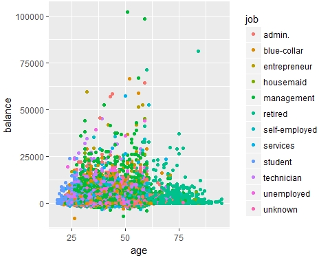
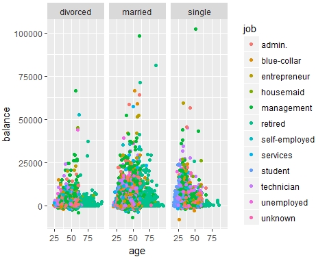
R provides excellent visualization features that are essential for exploring data before using it in automated learning. Applied Supervised Learning with R helps you cover the complete process of employing R to develop applications using supervised machine learning algorithms for your business needs. The book starts by helping you develop your analytical thinking to create a problem statement using business inputs and domain research. You will then learn different evaluation metrics that compare various algorithms, and later progress to using these metrics to select the best algorithm for your problem. After finalizing the algorithm you want to use, you will study the hyperparameter optimization technique to fine-tune your set of optimal parameters. The book demonstrates how you can add different regularization terms to avoid overfitting your model. By the end of this book, you will have gained the advanced skills you need for modeling a supervised machine learning algorithm that precisely fulfills your business needs.
Table of Contents (12 chapters)
Applied Supervised Learning with R
Preface

Data Visualization


An essential part of what we call Exploratory Data Analysis (EDA), more on this in Chapter 2, Exploratory Analysis of Data, is the ability to visualize data in a way that communicates insights elegantly and makes storytelling far more comprehensible. Not only does data visualization help us in communicating better insights, but it also helps with spotting anomalies. Before we get there, let's look at some of the most common visualizations that we often use in data analysis. All the examples in this section will be in ggplot2, a powerful package in R. Just like dplyr and plyr, ggplot2 is built on the Grammar of Graphics, which is a tool that enables us to describe the components of a graphic concisely.

Note

Good grammar will allow us to gain insight into the composition of complicated graphics and reveal unexpected connections between seemingly different graphics.

(Cox 1978) [Cox, D. R. (1978), "Some Remarks on the Role in Statistics of Graphical Methods," Applied Statistics, 27 (1), 4–9. [3,26].

Scatterplot

A scatterplot is a type of plot or mathematical diagram using Cartesian coordinates to display values for typically two variables for a set of data. If the points are color-coded, an additional variable can be displayed.

It is the most common type of chart and is extremely useful in spotting patterns in the data, especially between two variables. We will use our bank data again to do some EDA. Let's use the Portuguese bank direct campaign dataset for the visualizations:

df_bank_detail <- read.csv("bank-full.csv", sep = ';')

ggplot works in a layered way of stacking different elements of the plot. In the following example of this section, in the first layer, we provide the data to the ggplot() method and then map it with aesthetic details like x and y-axis, in the example, the age and balance values, respectively. Finally, to be able to identify some reasoning associated with few high bank balances, we added a color based on the type of job.

Execute the following command to plot the scatterplot of age and balance:

ggplot(data = df_bank_detail) +
  geom_point(mapping = aes(x = age, y = balance, color = job))

Figure 1.8: Scatterplot of age and balance.

From Figure 1.8, the distribution of bank balance with age looks much normal, with middle age showing a high bank balance whereas youngsters and old people are on the lower side of the spectrum.

Interestingly, some outlier values seem to be coming from management and retired professionals.

In data visualization, it's always tempting to see a graph and jump to a conclusion. A data visual is for consuming the data better and not for drawing causal inference. Usually, an interpretation by an analyst is always vetted by a business. Graphs that are aesthetically pleasing often tempt you to put it into presentation deck. So, next time a beautiful chart gets into your presentation deck, carefully analyze what you are going to say.

Scatter Plot between Age and Balance split by Marital Status

In this section, we will draw three scatter plots in a single plot between age and balance split by marital status (one for each single, divorced, and married individuals).

Now, you could split the distribution by marital status. The patterns seem to be consistent among the single, married, and divorced individuals. We used a method called facet_wrap() as the third layer in ggplot. It takes a marital variable as a formula:

ggplot(data = df_bank_detail) +
  geom_point(mapping = aes(x = age, y = balance, color = job)) +
  facet_wrap(~ marital, nrow = 1)

Figure 1.9: Scatter plot between age and balance split by marital status