
The required theory
In this section, you are going to learn the required theory that supports the SAX representation. However, keep in mind that this book is more practical than it is theoretical. If you want to learn the theory in depth, you should read the research papers mentioned in this chapter, as well as the forthcoming ones, and the Useful links section found at the end of each chapter. Thus, the theory is about serving our main purpose, which is the implementation of techniques and algorithms.
The operation and the details of SAX are fully described in a research paper titled Experiencing SAX: a novel symbolic representation of time series, which was written by Jessica Lin, Eamonn Keogh, Li Wei, and Stefano Lonardi. This paper (https://doi.org/10.1007/s10618-007-0064-z) was officially published back in 2007. You do not have to read all of it from the front cover to the back cover, but it is a great idea to download it and read the first pages of it, giving special attention to the abstract and the introduction section.
We will begin by explaining the terms PAA and SAX. PAA stands for Piecewise Aggregate Approximation. The PAA representation offers a way to reduce the dimensionality of a time series. This means that it takes a long time series and creates a smaller version of it that is easier to work with.
PAA is also explained in the Experiencing SAX: a novel symbolic representation of time series paper (https://doi.org/10.1007/s10618-007-0064-z). From that, we can easily understand that PAA and SAX are closely related, as the idea behind SAX is based on PAA. The SAX representation is a symbolic representation of time series. Put simply, it offers a way of representing a time series in a summary form, in order to save space and increase speed.
The difference between PAA and SAX
The main difference between PAA and the SAX representation is that PAA just calculates the mean values of a time series, based on a sliding window size, whereas the SAX representation utilizes those mean values and further transforms PAA to get a discrete representation of a time series (or subsequence). In other words, the SAX representation converts the PAA representation into something that is better to work with. As you will find out in a while, this transformation takes place with the help of breakpoints, which divide the numeric space of the mean values into subspaces. Each subspace has a discrete representation based on the given breakpoint values.
Both PAA and SAX are techniques for dimensionality reduction. SAX is going to be explained in much more detail in a while, whereas the discussion about PAA ends here.
The next subsection tells us why we need SAX.
Why do we need SAX?
Time series are difficult to search. The longer a time series (or subsequence) is, the more computationally intensive it is to search for it or compare it with another one. The same applies to working with indexes that index time series – iSAX is such an index.
To make things simpler for you, what we will do is take a subsequence with x elements and transform it into a representation with w elements, where w is much smaller than x. In strict terms, this is called dimensionality reduction, and it allows us to work with long subsequences using less data. However, once we decide that we need to work with a given subsequence, we need to work with it using its full dimensions – that is, all its x elements.
The next subsection talks about normalization, which, among other things, allows us to compare values at different scales.
Normalization
The first two questions you might ask are what normalization is and why we need it.
Normalization is the process of adjusting values that use different scales to a common scale. A simple example is comparing Fahrenheit and Celsius temperatures – we cannot do that unless we bring all values to the same scale. This is the simplest form of normalization.
Although various types of normalization exist, what is needed here is standard score normalization, which is the simplest form of normalization, because this is what is used for time series and subsequences. Please do not confuse database normalization and normal forms with value normalization, as they are totally different concepts.
The reasons that we introduce normalization into the process are as follows:
- The first and most important reason is that we can compare datasets that use a different range of values. A simple case is comparing Celsius and Fahrenheit temperatures.
- A side effect of the previous point is that data anomalies are reduced but not eliminated.
- In general, normalized data is easier to understand and process because we deal with values in a predefined range.
- Searching using an index that uses normalized values might be faster than when working with bigger values.
- Searching, sorting, and creating indexes is faster since values are smaller.
- Normalization is conceptually cleaner and easier to maintain and change as your needs change.
Another simple example that supports the need for normalization is when comparing positive values with negative ones. It is almost impossible to draw useful conclusions when comparing such different kinds of observations. Normalization solves such issues.
Although we are not going to need to, bear in mind that we cannot go from the normalized version of a subsequence to the original subsequence, so the normalization process is irreversible.
The following function shows how to normalize a time series with some help from the NumPy Python package:
def normalize(x):
     eps = 1e-6
     mu = np.mean(x)
     std = np.std(x)
     if std < eps:
           return np.zeros(shape=x.shape)
     else:
           return (x-mu)/std
The previous function reveals the formula of normalization. Given a dataset, the normalized form of each one of its elements is equal to the value of the observation, minus the mean value of the dataset over the standard deviation of the dataset – both these statistical terms are explained in The tsfresh Python package section of this chapter.
This is seen in the return value of the previous function, (x-mu)/std. NumPy is clever enough to calculate that value for each observation without the need to use a for loop. If the standard deviation is close to 0, which is simulated by the value of the eps variable, then the return value of normalize() is equal to a NumPy array full of zeros.
The normalize.py script, which uses the previously developed function that does not appear here, gets a time series as input and returns its normalized version. Its code is as follows:
#!/usr/bin/env python3
import sys
import pandas as pd
import numpy as np
def main():
     if len(sys.argv) != 2:
           print("TS")
           sys.exit()
     F = sys.argv[1]
     ts = pd.read_csv(F, compression='gzip', header = None)
     ta = ts.to_numpy()
     ta = ta.reshape(len(ta))
     taNorm = normalize(ta)
     print("[", end = ' ')
     for i in taNorm.tolist():
           print("%.4f" % i, end = ' ')
     print("]")
if __name__ == '__main__':
     main()
The last for loop of the program is used to print the contents of the taNorm NumPy array with a smaller precision in order to take up less space. To do that, we need to convert the taNorm NumPy array into a regular Python list using the tolist() method.
We are going to feed normalize.py a short time series; however, the script also works with longer ones. The output of normalize.py looks as follows:
$ ./normalize.py ts1.gz
[ -1.2272 0.9487 -0.1615 -1.0444 -1.3362 1.4861 -1.0620 0.7451 -0.4858 -0.9965 0.0418 1.7273 -1.1343 0.6263 0.3455 0.9238 1.2197 0.3875 -0.0483 -1.7054 1.3272 1.5999 1.4479 -0.4033 0.1525 1.0673 0.7019 -1.0114 0.4473 -0.2815 1.1239 0.7516 -1.3102 -0.6428 -0.3186 -0.3670 -1.6163 -1.2383 0.5692 1.2341 -0.0372 1.3250 -0.9227 0.2945 -0.5290 -0.3187 1.4103 -1.3385 -1.1540 -1.2135 ]
With normalization in mind, let us now proceed to the next subsection, where we are going to visualize a time series and show the visual difference between the original version and the normalized version of it.
Visualizing normalized time series
In this subsection, we are going to show the difference between the normalized and the original version of a time series with the help of visualization. Keep in mind that we usually do not normalize the entire time series. The normalization takes place on a subsequence level based on the sliding window size. In other words, for the purposes of this book, we will normalize subsequences, not an entire time series. Additionally, for the calculation of the SAX representation, we process the normalized subsequences based on the segment value, which specifies the parts that a SAX representation will have. So, for a segment value of 2, we split the normalized subsequence into two. For a segment value of 4, we split the normalized subsequence into four sets.
Nevertheless, viewing the normalized and original versions of a time series is very educational. The Python code of visualize_normalized.py, without the implementation of normalize(), is as follows:
#!/usr/bin/env python3
import sys
import pandas as pd
import matplotlib.pyplot as plt
import numpy as np
def main():
     if len(sys.argv) != 2:
           print("TS")
           sys.exit()
     F = sys.argv[1]
     ts = pd.read_csv(F, compression='gzip', header = None)
     ta = ts.to_numpy()
     ta = ta.reshape(len(ta))
     # Find its normalized version
     taNorm = normalize(ta)
     plt.plot(ta, label="Regular", linestyle='-', markevery=10, marker='o')
     plt.plot(taNorm, label="Normalized", linestyle='-.', markevery=10, marker='o')
     plt.xlabel('Time Series', fontsize=14)
     plt.ylabel('Values', fontsize=14)
     plt.legend()
     plt.grid()
     plt.savefig("CH02_01.png", dpi=300, format='png', bbox_inches='tight')
if __name__ == '__main__':
     main()
The plt.plot() function is called twice, plotting a line each time. Feel free to experiment with the Python code in order to change the look of the output.
Figure 2.1 shows the output of visualize_normalized.py ts1.gz, which uses a time series with 50 elements.
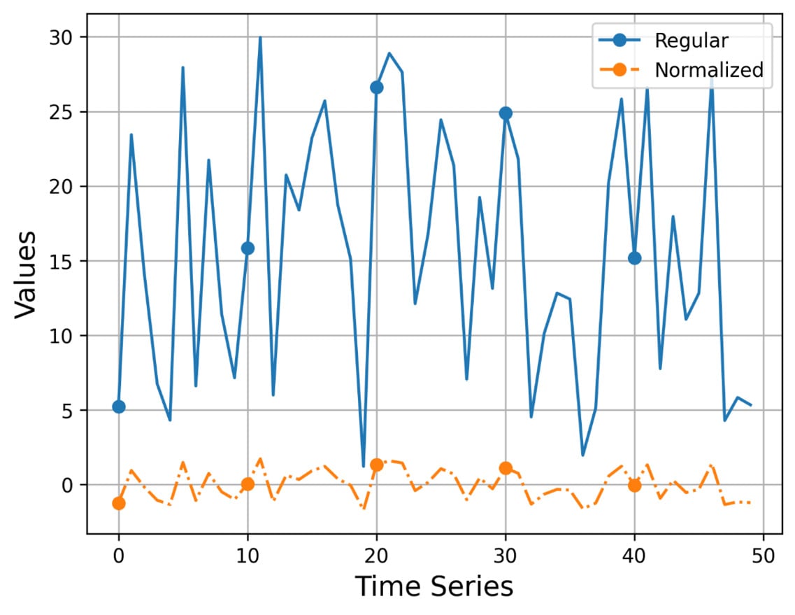
Figure 2.1 – The plotting of a time series and its normalized version
I think that Figure 2.1 speaks for itself! The values of the normalized version are located around the value of 0, whereas the values of the original time series can be anywhere! Additionally, we make the original time series smoother without completely losing its original shape and edges.
The next section is about the details of the SAX representation, which is a key component of every iSAX index.