An introduction to SAX

As mentioned previously, SAX stands for Symbolic Aggregate Approximation. The SAX representation was officially announced back in 2007 in the Experiencing SAX: a novel symbolic representation of time series paper (https://doi.org/10.1007/s10618-007-0064-z).

Keep in mind that we do not want to find the SAX representation of an entire time series. We just want to find the SAX representation of a subsequence of a time series. The main difference between a time series and a subsequence is that a time series is many times bigger than a subsequence.

Each SAX representation has two parameters named cardinality and the number of segments. We will begin by explaining the cardinality parameter.

The cardinality parameter

The cardinality parameter specifies the number of possible values each segment can have. As a side effect, the cardinality parameter defines the way the y axis is divided – this is used to get the value of each segment. There exist multiple ways to specify the value of a segment based on the cardinality. These include alphabet characters, decimal numbers, and binary numbers. In this book, we will use binary numbers because they are easier to understand and interpret, using a file with the precalculated breakpoints for cardinalities up to 256.

So, a cardinality of 4, which is 22, gives us four possible values, as we use 2 bits. However, we can easily replace 00 with the letter a, 01 with the letter b, 10 with the letter c, 11 with the letter d, and so on, in order to use letters instead of binary numbers. Keep in mind that this might require minimal code changes in the presented code, and it would be good to try this as an exercise when you feel comfortable with SAX and the provided Python code.

The format of the file with the breakpoints, which in our case supports cardinalities up to 256 and is called SAXalphabet, is as follows:

$ head -7 SAXalphabet
0
-0.43073,0.43073
-0.67449,0,0.67449
-0.84162,-0.25335,0.25335,0.84162
-0.96742,-0.43073,0,0.43073,0.96742
-1.0676,-0.56595,-0.18001,0.18001,0.56595,1.0676
-1.1503,-0.67449,-0.31864,0,0.31864,0.67449,1.1503

The values presented here are called breakpoints in the SAX terminology. The value in the first line divides the y axis into two areas, separated by the x axis. So, in this case, we need 1 bit to define whether we are in the upper space (the positive y value) or the lower one (the negative y value).

As we will use binary numbers to represent each SAX segment, there is no point in wasting them. Therefore, the values that we will use are the powers of 2, from 2 1 (cardinality 2) to 2 8 (cardinality 256).

Let us now present Figure 2.2, which shows how -0.67449, 0, 0.67449 divides the y axis, which is used in the 2 2 cardinality. The bottom part begins from the minus infinitive up to -0.67449, the second part from -0.67449 up to 0, the third part from 0 to 0.67449, and the last part from 0.67449 up to plus infinitive.

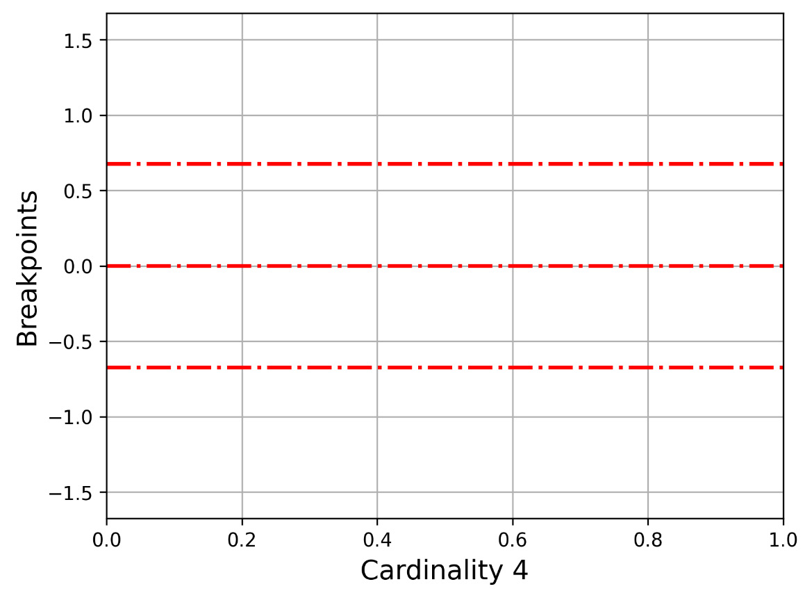
Figure 2.2 – The y axis for cardinality 4 (three breakpoints)

Let us now present Figure 2.3, which shows how -1.1503, -0.67449, -0.31864, 0, 0.31864, 0.67449, 1.1503 divides the y axis. This is for the 2 3 cardinality.

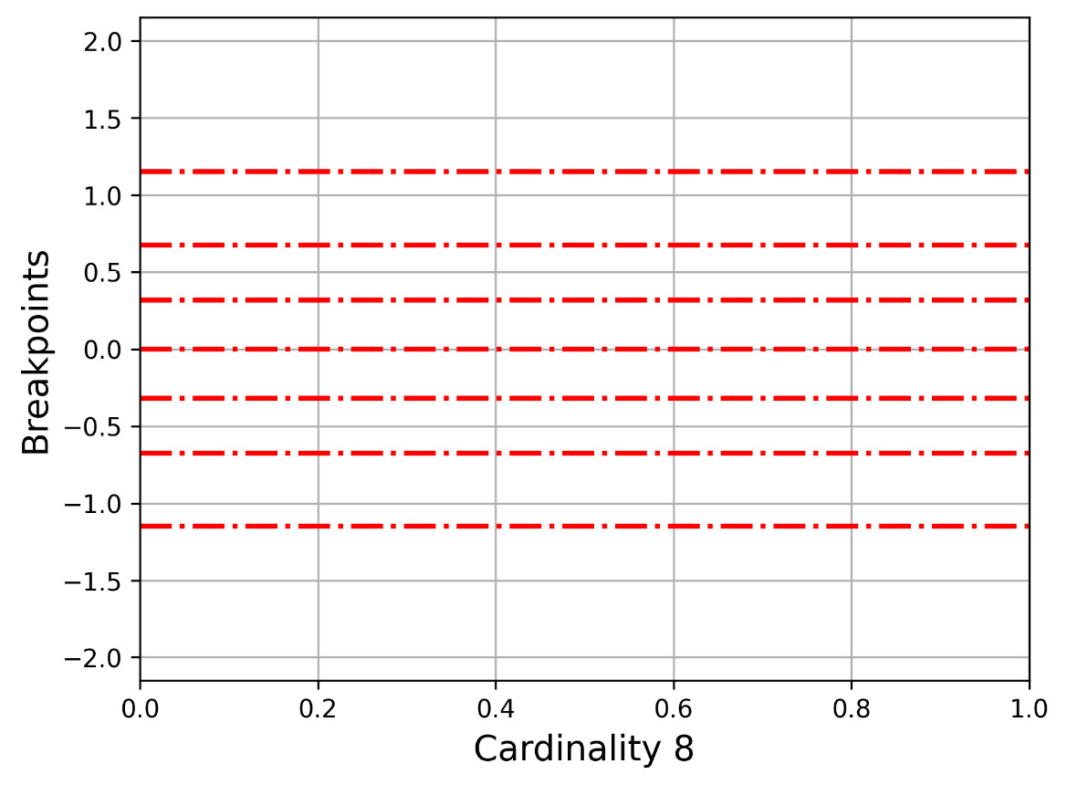
Figure 2.3 – The y axis for cardinality 8 (7 breakpoints)

As this can be a tedious job, we have created a utility that does all the plotting. Its name is cardinality.py, and it reads the SAXalphabet file to find the breakpoints of the desired cardinality before plotting them.

The Python code for cardinality.py is as follows:

#!/usr/bin/env python3
import sys
import pandas as pd
import matplotlib.pyplot as plt
import numpy as np
import os
breakpointsFile = "./sax/SAXalphabet"
def main():
     if len(sys.argv) != 3:
           print("cardinality output")
           sys.exit()
     n = int(sys.argv[1]) - 1
     output = sys.argv[2]
     path = os.path.dirname(__file__)
     file_variable = open(path + "/" + breakpointsFile)
     alphabet = file_variable.readlines()
     myLine = alphabet[n - 1].rstrip()
     elements = myLine.split(',')
     lines = [eval(i) for i in elements]
     minValue = min(lines) - 1
     maxValue = max(lines) + 1
     fig, ax = plt.subplots()
     for i in lines:
           plt.axhline(y=i, color='r', linestyle='-.', linewidth=2)
     xLabel = "Cardinality " + str(n)
     ax.set_ylim(minValue, maxValue)
     ax.set_xlabel(xLabel, fontsize=14)
     ax.set_ylabel('Breakpoints', fontsize=14)
     ax.grid()
     fig.savefig(output, dpi=300, format='png', bbox_inches='tight')
if __name__ == '__main__':
     main()

The script requires two command-line parameters – the cardinality and the output file, which is used to save the image. Note that a cardinality value of 8 requires 7 breakpoints, a cardinality value of 32 requires 31 breakpoints, and so on. Therefore, the Python code for cardinality.py decreases the line number that it is going to search for in the SAXalphabet file to support that functionality. Therefore, when given a cardinality value of 8, the script is going to look for the line with 7 breakpoints in SAXalphabet. Additionally, as the script reads the breakpoint values as strings, we need to convert these strings into floating-point values using the lines = [eval(i) for i in elements] statement. The rest of the code is related to the Matplotlib Python package and how to draw lines using plt.axhline().

The next subsection is about the segments parameter.

The segments parameter

The (number of) segments parameter specifies the number of parts (words) a SAX representation is going to have. Therefore, a segments value of 2 means that the SAX representation is going to have two words, each one using the specified cardinality. Therefore, the values of each part are determined by the cardinality.

A side effect of this parameter is that, after normalizing a subsequence, we divide it by the number of segments and work with these different parts separately. This is the way the SAX representation works.

Both cardinality and segments values control the data compression ratio and the accuracy of the subsequences of a time series and, therefore, the entire time series.

The next subsection shows how to manually compute the SAX representation of a subsequence – this is the best way to fully understand the process and be able to identify bugs or errors in the code.

How to manually find the SAX representation of a subsequence

Finding the SAX representation of a subsequence looks easy but requires lots of computations, which makes the process ideal for a computer. Here are the steps to find the SAX representation of a time series or subsequence:

1. First, we need to have the number of segments and the cardinality.
2. Then, we normalize the subsequence or the time series.
3. After that, we divide the normalized subsequence by the number of segments.
4. For each one of these parts, we find its mean value.
5. Finally, based on each mean value, we calculate its representation based on the cardinality. The cardinality is what defines the breakpoint values that are going to be used.

We will use two simple examples to illustrate the manual computation of the SAX representation of a time series. The time series is the same in both cases. What will be different are the SAX parameters and the sliding window size.

Let’s imagine we have the following time series and a sliding window size of 4:

{-1, 2, 3, 4, 5, -1, -3, 4, 10, 11, . . .}

Based on the sliding window size, we extract the first two subsequences from the time series:

• S1 = {-1, 2, 3, 4}
• S2 = {2, 3, 4, 5}

The first step that we should take is to normalize these two subsequences. For that, we will use the normalize.py script we developed earlier – we just have to save each subsequence into its own plain text file and compress it using the gzip utility, before giving it as input to normalize.py. If you use a Microsoft Windows machine, you should look for a utility that allows you to create such ZIP files. An alternative is to work with plain text files, which might require some small code changes in the pd.read_csv() function call.

The output of the normalize.py script when processing S1 (s1.txt.gz) and S2 (s2.txt.gz) is the following:

$ ./normalize.py s1.txt.gz
[ -1.6036 0.0000 0.5345 1.0690 ]
$ ./normalize.py s2.txt.gz
[ -1.3416 -0.4472 0.4472 1.3416 ]

So, the normalized versions of S1 and S2 are as follows:

• N1 = {-1.6036, 0.0000, 0.5345, 1.0690}
• N2 = {-1.3416, -0.4472, 0.4472, 1.3416}

In this first example, we use a segments value of 2 and a cardinality value of 4 (22). A segment value of 2 means that we must divide each normalized subsequence into two parts. These two parts contain the following data, based on the normalized versions of S1 and S2:

• For S1, the two parts are {-1.6036, 0.0000} and {0.5345, 1.0690}
• For S2, the two parts are {-1.3416, -0.4472} and {0.4472, 1.3416}

The mean values of each part are as follows:

• For S1, they are -0.8018 and 0.80175
• For S2, they are -0.8944 and 0.8944

For the cardinality of 4, we are going to look at Figure 2.2 and the respective breakpoints, which are -0.67449, 0, and 0.67449. So, the SAX values of each segment are as follows:

• For S1, they are 00 because -0.8018 falls at the bottom of the plot and 11
• For S2, they are 00 and 11 because 0.8944 falls at the top of the plot

Therefore, the SAX representation of S1 is [00, 11] and for S2, it is [00, 11]. It turns out that both subsequences have the same SAX representation. This makes sense, as they only differ in one element, which means that their normalized versions are similar.

Note that in both cases, the lower cardinality begins from the bottom of the plot. For Figure 2.2, this means that 00 is at the bottom of the plot, 01 is next, followed by 10, and 11 is at the top of the plot.

In the second example, we will use a sliding window size of 8, a segments value of 4, and a cardinality value of 8 (23).

About the sliding window size

Keep in mind that the normalized representation of the subsequence remains the same when the sliding window size remains the same. However, if either the cardinality or the segments change, the resulting SAX representation might be completely different.

Based on the sliding window size, we extract the first two subsequences from the time series – S1 = {-1, 2, 3, 4, 5, -1, -3, 4} and S2 = {2, 3, 4, 5, -1, -3, 4, 10}.

The output of the normalize.py script is going to be the following:

$ ./normalize.py T1.txt.gz
[ -0.9595 0.1371 0.5026 0.8681 1.2337 -0.9595 -1.6906 0.8681 ]
$ ./normalize.py T2.txt.gz
[ -0.2722 0.0000 0.2722 0.5443 -1.0887 -1.6330 0.2722 1.9052 ]

So, the normalized versions of S1 and S2 are N1 = {-0.9595, 0.1371, 0.5026, 0.8681, 1.2337, -0.9595, -1.6906, 0.8681} and N2 = {-0.2722, 0.0000, 0.2722, 0.5443, -1.0887, -1.6330, 0.2722, 1.9052}, respectively.

A segment value of 4 means that we must divide each one of the normalized subsequences into four parts. For S1, these parts are {-0.9595, 0.1371}, {0.5026, 0.8681}, {1.2337, -0.9595}, and {-1.6906, 0.8681}.

For S2, these parts are {-0.2722, 0.0000}, {0.2722, 0.5443}, {-1.0887, -1.6330}, and {0.2722, 1.9052}.

For S1, the mean values are -0.4112, 0.68535, 0.1371, and -0.41125. For S2, the mean values are -0.1361, 0.40825, -1.36085, and 1.0887.

About the breakpoints of the cardinality value of 8

Just a reminder here that for the cardinality value of 8, the breakpoints are (000) -1.1503, (001) -0.67449, (010) -0.31864, (011) 0, (100) 0.31864, (101) 0.67449, and (110) 1.1503 (111). In parentheses, we present the SAX values for each breakpoint. For the first breakpoint, we have the 000 value to its left and 001 to its right. For the last breakpoint, we have the 110 value to its left and 111 to its right. Remember that we use seven breakpoints for a cardinality value of 8.

Therefore, the SAX representation of S1 is ['010', '110', '100', '010'], and for S2, it is['011', '101', '000', '110']. The use of single quotes around SAX words means that internally we store SAX words as strings, despite the fact that we calculate them as binary numbers because it is easier to search and compare strings.

The next subsection examines a case where a subsequence cannot be divided perfectly by the number of segments.

Ηow can we divide 10 data points into 3 segments?

So far, we have seen examples where the length of the subsequence can be perfectly divided by the number of segments. However, what happens if that is not possible?

In that case, there exist data points that contribute to two adjacent segments at the same time. However, instead of putting the whole point into a segment, we put part of it into one segment and part of it into another!

This is further explained on page 18 of the Experiencing SAX: a novel symbolic representation of time series paper. As stated in the paper, if we cannot divide the sliding window length by the number of segments, we can use a part of a point in a segment and a part of a point in another segment. We do that for points that are between two segments and not for any random points. This can be explained using an example. Imagine we have a time series such as T = {t1, t2, t3, t4, t5, t6, t7, t8, t9, t10}. For the S1 segment, we take the values of {t1, t2, t3} and one-third of the value of t4. For the S2 segment, we take the values of {t5, t6} and two-thirds of the values of t4 and t7. For the S3 segment, we take the values of {t8, t9, t10} and the third of the value of t7 that we have not used so far. This is also explained in Figure 2.4:

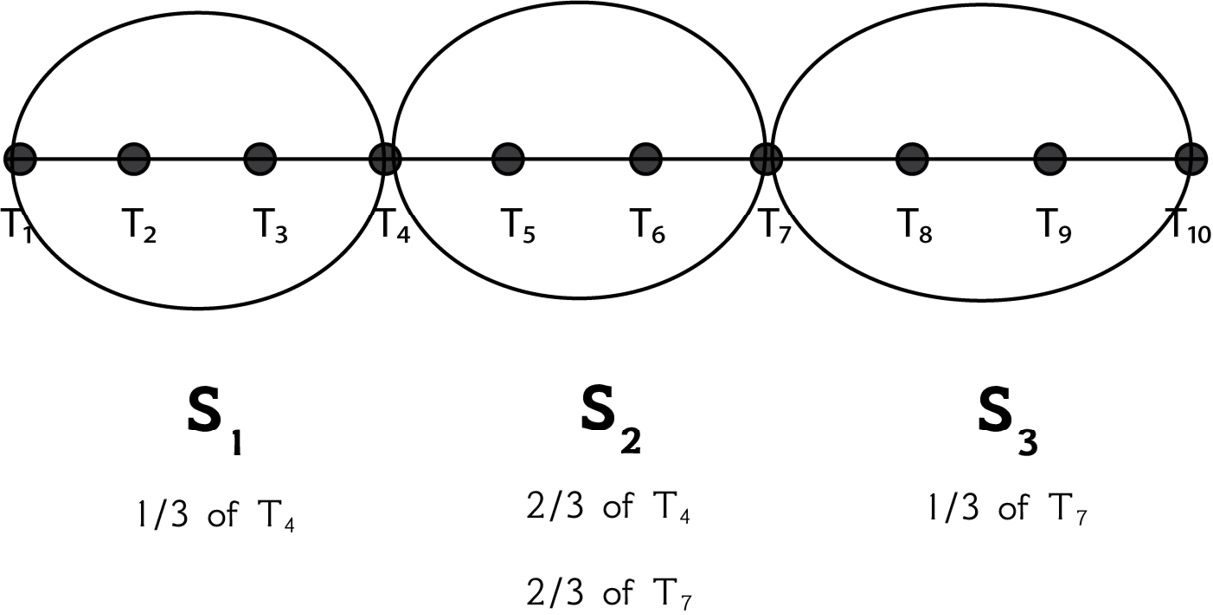
Figure 2.4 – Dividing 10 data points into 3 segments

Put simply, this is a convention decided by the creators of SAX that applies to all cases where we cannot perfectly divide the number of elements by that of the segments.

In this book, we will not deal with that case. The sliding window size, which is the length of the generated subsequences, and the number of segments are both part of a perfect division, with a remainder of 0. This simplification does not change the way SAX works, but it makes our lives a little easier.

The subject of the next subsection is how to go from higher cardinalities to lower ones without doing every computation.

Reducing the cardinality of a SAX representation

The knowledge gained from this subsection will be applicable when we discuss the iSAX index. However, as what you will learn is directly related to SAX, we have decided to discuss it here first.

Imagine that we have a SAX representation at a given cardinality and that we want to reduce the cardinality. Is that possible? Can we do this without calculating everything from scratch? The answer is simple – this can be done by ignoring trailing bits. Given a binary value of 10,100, the first trailing bit is 0, then the next trailing bit is 0, then 1, and so on. So, we start from the bits at the end, and we remove them one by one.

As most of you, including me when I first read about it, might find this unclear, let me show you some practical examples. Let us take the following two SAX representations from the How to manually find the SAX representation of a subsequence subsection of this chapter – [00, 11] and [010, 110, 100, 010]. To convert [00, 11] into the cardinality of 2, we must just delete the digits at the end of each SAX word. So, the new version of [00, 11] will be [0, 1]. Similarly, [010, 110, 100, 010] is going to be [01, 11, 10, 01] for the cardinality of 4 and [0, 1, 1, 0] for the cardinality of 2.

So, from a higher cardinality – a cardinality with more digits – we can go to a lower cardinality by subtracting the appropriate number of digits from the right side of one or more segments (the trailing bits). Can we go in the opposite direction? Not without losing accuracy, but that would still be better than nothing. However, generally, we don’t go in the opposite direction. So far, we know the theory regarding the SAX representation. The section that follows briefly explains the basics of Python packages and shows the development of our own package, named sax.