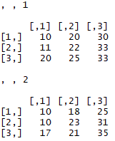
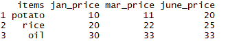
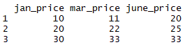
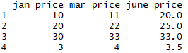
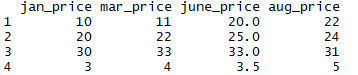
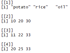
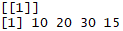
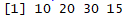
Before we start delving deep into R for geospatial analysis, we need to have a good understanding of how R handles and stores different types of data. We also need to know how to undertake different operations on that data.

There are three main data types in R, and they are as follows:

• Numerics
• Logical or Boolean
• Character

Numerics are any numbers with decimal values; thus, 21.0 and 21.1 are both numerics. We can use addition, subtraction, multiplication, division, and so on, with these numerics. Interestingly, R also considers integer numbers to be numerics. Logical or Boolean data consists of TRUE and FALSE; they are mainly used for different comparisons. The character variable consists of text, such as the name of something. We write character values in R by putting our character values inside "", or double quotes.

Just before digging any deeper, we need to know how to assign values to any variable. So, what is a variable? It's like a container, which holds different value(s) of different types (or the same type). When assigning multiple values to any variable, we write the variable name to the left, followed by an <- or = and then the value. So, if we want to assign 2 to a variable x, we can write either of the two:

x <- 2

or

x = 2

The data structures in R are as follows:

• Vectors
• Matrices
• Arrays
• Data frames
• Lists
• Factors

Vectors are used to store single or multiple values of similar data types in a variable and are considered to be one-dimensional arrays. That means that the x variable we just defined is a vector. If we want to create a vector with multiple numeric values, we assign as before with one additional rule: we put all the values inside c() and separate all the values with , except the last value. Let's look at an example:

val = c(1, 2, 3, 4, 5, 6)

What happens if we mix different data types such as both numerics and characters? It works! (A variable's name is arbitrarily named as val, but you can name your variable anything that you feel appropriate, anything!) Except in some cases, such as variable names, shouldn't start with any special character:

x = c(1, 2.0, 3.0, 4, 5, "Hello", "OK")

What we have just learned about storing data of the same types doesn't seem to be true then, right? Well, not exactly. What R does behind the scenes is that it tries to convert all the values mentioned for the x variable to the same type. As it can't convert Hello and OK to numeric types, for conformity it converts all the numeric values 1, 2.0, 3.0, 4, and 5 to character values: that is, "1", "2.0", "3.0", "4", and "5", and adds two more values, "Hello" and "OK", and assigns all these character values to x. We can check the class (data type) of a variable in R with class(variable_name), and let's confirm that x is indeed a character variable:

class(x)

We will see that the R window will show the following output:

[1] "character"

We can also label vectors or give names to different values according to our need. Suppose we want to assign temperature values recorded at different times to a variable with a recorded time as a label. We can do so using this code:

temperature = c(morning = 20, before_noon = 23, after_noon = 25, evening = 22, night =  18)

Suppose the prices of three commodities, namely potatoes, rice, and oil were $10, $20, and $30 respectively in January 2018, denoted by the vector jan_price, and the prices of all these three elements increased by $1, $2, and $3 respectively in March 2018, denoted by the vector increase. Then, we can add two vectors mar_price and increase to get the new price as follows:

jan_price = c(10, 20, 30)
increase = c(1, 2, 3)
mar_price = jan_price + increase

To see the contents of mar_price, we just need to write it and then press Enter:

mar_price

We now see that mar_price is updated as expected:

[1] 11 22 33

Similarly, we can subtract and multiply. Remember that R uses element-wise computation, meaning that if we multiply two vectors which are of the same size, the first element of the first vector will be multiplied by the first element of the second vector, and the second element of the second vector will be multiplied by the second element of the second vector, and as such:

x = c(10, 20, 30)
y = c(1, 2, 3)
x * y

The result of this multiplication is this:

[1] 10 40 90

If we multiply a vector with multiple values by a single value, that latter value multiplies every single element of the vector separately. This is demonstrated in the following example:

x * 2

We can see the output of the preceding command as follows:

[1] 20 40 60

As a vector does element-wise computation, if we check for any condition, the condition will be checked for each element. Thus, if we want to know which values in x are greater than 15:

x > 15

As the second and third elements satisfy this condition of being greater than 15, we see TRUE for these positions and FALSE for the first position as follows:

[1] FALSE TRUE TRUE

Indexing in R or the first element of any data type starts with 1; thus, the third or fourth element in R can be accessed with index 3 or 4. We need to access any particular index of a variable with a variable name followed by the index inside []. Thus, the third element of x can be accessed as follows:

x[3]

By pressing Enter after x[3], we see that the third element of x is this:

30

If we want to select all items but the third one, we need to use - in the following way:

x[-3]

We now see that x has all of the elements except the third one:

[1] 10 20

Suppose, we also have the prices of these three items for the month of June as follows:

june_price = c(20, 25, 33)

Now if we want to stack all these three months in a single variable, we can't use vectors anymore; we need a new data structure. One of the data structures to rescue in this case is the matrix. A matrix is basically a two-dimensional array of data elements with a number of rows and columns fixed. Like a vector, a matrix can also contain just one type of element; a mix of two types is not allowed. To combine these three vectors with every row corresponding to a particular month's prices of different items and every column corresponding to prices of different items in a particular month, what we can do is first combine these three vectors inside a matrix() command, followed by a comma and nrow = 3, indicating the fact that there are three different items (for example, items are arranged row-wise and months are arranged column-wise).

all_prices = matrix(c(jan_price, mar_price, june_price), nrow= 3)
all_prices

The all_prices data frame will look like the following:

[,1] [,2] [,3]
 [1,] 10 11 20
 [2,] 20 22 25
 [3,] 30 33 33

Now suppose we change our mind and want to arrange this with the items displayed column-wise and the prices displayed row-wise; that is, the first row corresponds to the prices of different items in a particular month and the first column corresponds to the first month's (January's) prices of different items, with that arrangement continuing for every other row and column. We can do so very easily by mentioning byrow = TRUE inside the matrix. byrow = TRUE arranges the values of vectors row-wise. It arranges the matrix by aligning all the elements row-wise allowing for its dimensions:

all_prices2 = matrix(c(jan_price, mar_price, june_price), nrow= 3, byrow = TRUE)  
all_prices2

The output will look like the following:

[,1] [,2] [,3]
 [1,] 10 20 30
 [2,] 11 22 33
 [3,] 20 25 33

We can see that here jan_price is considered as the first row, mar_price as the second row, and june_price as the third row in all_prices2.

Arrays are also like matrices, but they allow us to have more than two dimensions. The all_prices2 row has prices of different items for January, March, and June 2018. Now, suppose we also want to record prices for 2017. We can do so by using array() and in this case we want to add two 3x3 matrices where the first one corresponds to 2018 and the latter matrix corresponds to 2017. In array(m, n, p), m and n stand for the dimensions of the matrix and p stands for how many matrices we want to store.

In the following example, we define six vectors for three different months for two different years. Now we create an array by combining six different vectors using c() and by using them inside array() as inputs as follows:

# Create six vectors
jan_2018 = c(10, 11, 20)
mar_2018 = c(20, 22, 25)
june_2018 = c(30, 33, 33)
jan_2017 = c(10, 10, 17)
mar_2017 = c(18, 23, 21)
june_2017 = c(25, 31, 35)

# Now combine these vectors into array
combined = array(c(jan_2018, mar_2018, june_2018, jan_2017, mar_2017, june_2017),dim = c(3,3,2))
combined

We can now see that we have two matrices of 3 x 3 dimensions, as in the output as follows:

Data frames are like matrices, except for the one additional advantage that we can now have a mix of different element types in a data frame. For example, we can now store both numeric and character elements in this data structure. Now, we can also put the names of different food items along with their prices in different months to be stored in a data frame. First, define a variable with the names of different food items:

items = c("potato", "rice", "oil")

We can define a data frame using data.frame as follows:

all_prices3 = data.frame(items, jan_price, mar_price, june_price) 
all_prices3

The data frame all_prices3 looks like the following:

Accessing elements in a data frame can be done by using either [[]] or $. To select all the values of mar_price or the second column, we can do either of the two methods provided as follows:

all_prices3$mar_price

This gives the values of the mar_price column of the all_prices3 data frame:

[1] 11 22 33

Similarly, there is the following:

all_prices3[["mar_price"]]

We now find the same output as we found by using the $ sign:

[1] 11 22 33

We can also use [] to access a data frame. In this case, we can utilize both the row and column dimensions to access an element (or elements) using the row index indicated by the number before, and the column index indicated by the number after. For example, if we wanted to access the second row and third column of all_prices3, we would write this:

 all_prices3[2, 3]

This gives the following output:

[1] 22

Here, for simplicity, we will drop items column from all_prices3 using - and rename the new variable as all_prices4 and we can define this value in a new vector pen as follows:

  all_prices4 = all_prices3[-1]
all_prices4

We can now see that the items column is dropped from the all_prices4 data frame:

We can add a row using rbind(). Now we define a new numerical vector that contains the price of the pen vector for January, March, and June, and we can add this row using rbind():

pen = c(3, 4, 3.5)
all_prices4 = rbind(all_prices4, pen)
all_prices4

Now we see from the following output that a new observation is added as a new row:

We can add a column using cbind(). Now, suppose we also have information on the prices of potato, rice, oil, and pen for August as given in the vector aug_price:

aug_price = c(22, 24, 31, 5)

We can now use cbind() to add aug_price as a new column to all_prices4:

all_prices4 = cbind(all_prices4, aug_price)
all_prices4

Now all_prices4 has a new column aug_price added to it:

Now, items jan_price and mar_price have four elements, whereas june_price has three elements. So, we can't use a data frame in this case to store all of these values in a single variable. Instead, we can use lists. Using lists, we can get almost all the advantages of a data frame in addition to its capacity for storing different sets of elements (columns in the case of data frames) with different lengths:

all_prices_list2 = list(items, jan_price, mar_price, june_price)
all_prices_list2

We can now see that all_prices_list2 has a different structure than that of a data frame:

Accessing list elements can be done by either using [] or [[]] where the former gives back a list and the latter gives back element(s) in its original data type. We can get the values of jan_price in the following way:

all_prices_list2[2]

Using [], we are returned with the second element of all_prices_list2 as a list again:

Note that, by using [], what we get back is another list and we can't use different mathematical operations on it directly.

class(all_prices_list2[2])

We can see, as follows, that the class of all_prices_list2 is a list:

We can get this data in original data types (that is, a numeric vector) by using [[]] instead of []:

all_prices_list2[[2]]

Now, we get the second element of the list as a vector:

We can see that it is numeric and we can check further to confirm that it is numeric:

class(all_prices_list2[[2]])

The following result confirms that it is indeed a numeric vector:

We can also create categorical variables with factor().

Suppose we have a numeric vector x and we want to convert it to a factor, we can do so by following the code as shown as follows:

x = c(1, 2, 3)
x = factor(x)
class(x)

We now see that the class is a factor, as we can see in the following output:

[1] "factor"

Now, we can also look at the internal structure of this vector x, using str() as follows:

str(x)

We now see that it converts 1, 2, and 3 to factors:

[1]  Factor w/ 3 levels "1", "2", "3": 1 2 3