R is a programming language intended for use for statistical analysis. Additionally, it can be utilized in an object-oriented or functional way. Specifically, it is an implementation of S, an interactive statistical programming language. R was initially released in August 1993. It is maintained today by the R Development Core Team.

RStudio is an incredibly useful Integrated Development Environment (IDE) for writing and using R. Many data scientists use RStudio for writing R, as it provides a console window, a code editor, tools to help create plots and graphics, and can even be integrated with GitHub to support version control.

While R does share some functionality with Microsoft Excel, it allows you to have more control over your data, and you can add on a variety of packages that allow statistical functionality out of the box—you won't have to build a formula to conduct a survival analysis; you can just install the survival package and use that!

Out of the box, R is completely usable. Open R on your machine. Let's use R for some basic arithmetic such as addition, multiplication, subtraction, and division. The following screenshot demonstrates this:

It also provides functions such as sum() and sqrt() for addition and calculation of the square root. The following screenshot shows this in action:

R can—and will—do basic arithmetic like a calculator, using symbols you're familiar with. One you may not have used before is exponentiate, where you use two asterisks, for example, 4 ** 2, which you can read as 4 to the power of 2.

Once you want to start doing math beyond basic arithmetic, such as finding square roots or summing many numbers, you have to start using functions.

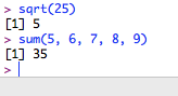
Let's now try and execute the sum() and sqrt() functions in R. Follow the steps given below:

1. Open the R console on your system.
2. Type the code as follows:

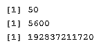
sum(1, 2, 3, 4, 5)
sqrt(144)

3. Execute the code.

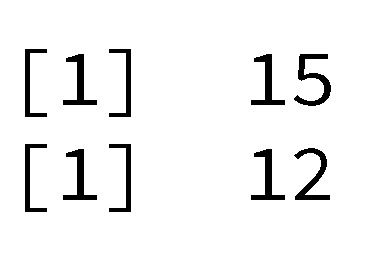
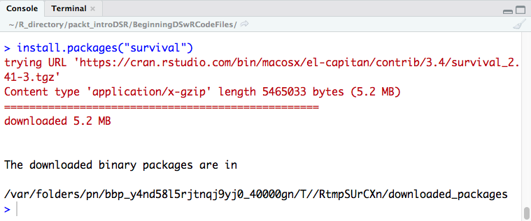
Output: The preceding code provides the following output:

Functions such as sum() and sqrt() are called base functions, which are built into R. This means that they come pre-installed when R is downloaded.

We could build all of our code right in the R console, but eventually, we might want to see our files, a list of everything in our global environment, and more, so instead, we'll use RStudio. Close R, and when it asks you to save the workspace image, for now, click Don't Save. (More explanation on workspace images and saving will come later in this chapter.)

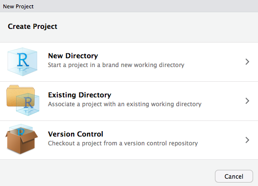
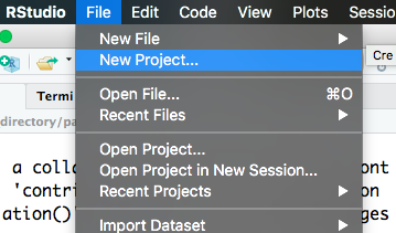
Open RStudio. We'll use RStudio for all of our code development from here on. One major benefit of RStudio is that we can use Projects, which will organize all of the files for analysis in one folder on our computer automatically. Projects will keep all of the parts of your analysis organized in one space in a chosen folder on your machine. Any time you start a new project, you should start a new project in RStudio by going to File | New Project, as shown in the below screenshot, or by clicking the new project button (blue, with a green plus sign ).

Creating a project from a New Directory allows us to create a folder on our drive (here E:\) to store all code files, data, and anything else associated with the book. If there was an existing folder on our drive that we'd like to make the directory for the project, we would choose the Existing Directory option. The Version Control option allows you to clone a repository from GitHub or another version control site. It makes a copy of the project stored on GitHub and saves it on your computer:

The working directory in R is the folder where all of the code files and output will be saved. It should be the same as the folder you choose when you create a project from a new or existing directory. To verify the working directory at any time, use the getwd() function. It will print the working directory as a character string (you can tell because it has quotation marks around it). The working directory can be changed at any time by using the following syntax:

setwd("new location/on the/computer")

To create a new script in R, navigate to File | New File | R Script, as shown in the screenshot below, or click the button on the top left that looks like a piece of paper with a green arrow on it .

Inside New File, there are options to create quite a few different things that you might use in R. We'll be creating R scripts throughout this book.

Custom functions are fairly straightforward to create in R. Generally, they should be created using the following syntax:

name_of_function <- function(input1, input2){
operation to be performed with the inputs
}

The example custom function is as follows:

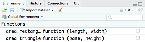
area_triangle <- function(base, height){
0.5 * base * height
}

Once the custom function code has been run, it will display in the Global Environment in the upper right corner and is now available for use in your RStudio project, as shown in the following screenshot:

One crucial step upon exiting RStudio or when you close your computer is to save a copy of the global environment. This will save any data or custom functions in the environment for later use and is done with the save.image() function, into which you'll need to enter a character string of what you want the saved file to be called, for example, introDSwR.RData. It will always be named with the extension .RData. If you were to open your project again some other time and want to load the saved environment, you use the load() function, with the same character string inside it.

Let us now set up a new project that we will use throughout the book. We will create an R project, script, custom function, and save an image of the global environment. Follow the steps given below:

1. Open RStudio.
2. Navigate to File | New Project to start a new project:
   • Start with a new directory and save it in a place on your computer that makes sense to you.
   • Save the project with the name IntroToDSwRCourse.
3. Check the working directory using the getwd() function and be sure it's the same folder you chose to save your project in.
4. Start a new script. Save the script with the filename lesson1_exercise.R.
5. Write a custom function, area_rectangle(), which calculates the area of a rectangle, with the following code:

area_rectangle <- function(length, width){
length * width
}

6. Try out area_rectangle() with the following sets of lengths and widths:
   • 5, 10
   • 80, 7
   • 48209302930, 4

The code will be as follows:

area_rectangle(5, 10)
area_rectangle(80, 70)
area_rectangle(48209302930, 4)

7. Save an image of the global environment for later; name the file introToDSwR.RData.

Output: The output you get after executing the getwd() function will be the folder on your computer that you have chosen to save your project in.

The area of the rectangle with different lengths will be provided as follows:

R and RStudio will be our main tools throughout this book for statistical analysis and programming. We've now seen how to create a new project, a new R script, and how to save a workspace image for use later.

In this chapter, we've already seen some of the base functions that are built into R. We also built a few custom functions, area_triangle() and area_rectangle(), in the last section.

Now, let's talk about packages. Anyone can write an R package of useful functions and publish it for use by others. Packages are usually made available on the Comprehensive R Archive Network (CRAN) website, or Bioconductor, a collection of packages for bioinformatics and other uses. Both these sites conduct a thorough review of submitted packages before publishing them on their sites, so package developers often keep beta versions of packages, or those that are useful but may not pass the inspections, on GitHub.

RStudio makes installing packages very easy. There are two ways to do so: either type install.packages("package_name") in a script or your console, or you can navigate to the Packages tab in the lower right window and click Install, which will show a window that allows you to type the names of the packages that are available on CRAN. You can even install multiple packages if you separate them with a comma. You'll want to keep Install dependencies checked, as this will install any packages that the package you've chosen depends on to run successfully—you'll want those! Let's see this in the following screenshot:

Let's now use two different methods to install R packages. Follow these steps:

• Install the survival package using the following code:

install.packages("survival")

• Install the mice package using the Install button on the Packages tab.

Output: The following should be displayed on your console:

The same information should be displayed once you install mice, with that package's name subbed in for survival.

R and RStudio, plus its packages, are incredibly helpful data science tools that will be the focus of this book. Now, let's get your project for the book set up, and install a set of incredibly useful packages called the Tidyverse, for use throughout the rest of this book.

Scenario

You have been assigned the task of developing a report using R. You need to install the Tidyverse packages to develop that report.

Aim

To install Tidyverse, a set of useful packages that will be used later in the book. Load the inbuilt datasets into the project.

Prerequisites

Make sure that you have R and RStudio installed on your machine.

Steps for completion

1. Install the Tidyverse package using the install.package() function.

2. Load the ggplot2 library and the built-in msleep dataset.

3. Save the global image of the environment for use later use.

This activity was crucial. We've added a dataset and the Tidyverse packages to the project we intend to use for the rest of the book. We've also saved a copy of our global environment to our working directory. The Tidyverse packages, dplyr, ggplot2, tidyr, and a few others, will be very helpful throughout this book and in your data science work.