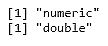
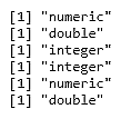
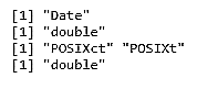
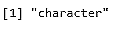
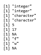
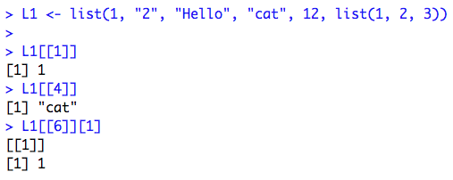
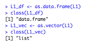
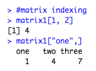
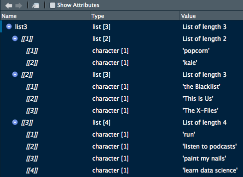
In this section, we'll begin first with an exploration of different variable types: numeric, character, and dates. We'll then look at different data structures in R: vectors, lists, matrices, and data frames.

Variable types exist in all programming languages and will tell the computer how to store and access a variable.

First, know that all variables created in R will have a class and a type. You can look at the class or type of anything in R using the class() and typeof() functions, respectively.

The class of an object is a broad designation, for example, character, numeric, integer, and date. These are very broad categories, and type elaborates more specifically on what type of variable it is, for example, a variable of class date can be of type character or POSIXct, depending on how it is stored. Type drills down into the details of a variable and how it's been stored in R, though sometimes class and type can be the same. For example, integers are of class and type integer, and character strings are of type and class character. Let's examine the following code snippet:

x <- 4.2
class(x)
typeof(x)

The preceding code provides the following output:

In this snippet, x has a class numeric, because it is a number, but also has a type double because it is a decimal number. This is because all numeric data in R is of type double unless the object has been explicitly declared to be an integer. Let's look at some examples of different classes and types.

The numeric data class includes all numbers except integers, which are their own separate class in R. Anything of class numeric will be of type double, unless it is explicitly declared as an integer. To create an integer, you must type a capital letter, L, after a whole number.

Let's now create and check the class() and typeof() of different numeric objects in R. Follow the steps given below:

1. Create the following numeric objects:

x <- 12.7
y <- 8L
z <- 950

2. Check the class and type of each using class() and typeof(), respectively, as follows:

class(x)
typeof(x)

class(y)
typeof(y)

class(z)
typeof(z)

Output: The preceding code provides the following output:

Character data is always mentioned in quotation marks; anything contained in quotation marks is called a character string. Usually, character data is of both class and type character.

Let's create and check the class() and typeof() of different character objects in R. Follow the steps given below:

1. Create the following objects:

a <- "apple"
b <- "7"
c <- "9-5-2016"

2. Check the class and type of each using class() and typeof(), respectively, as follows:

class(a)
typeof(a)

class(b)
typeof(b)

class(c)
typeof(c)

Output: The preceding code provides the following output:

Dates are a special type of data in R, and are distinct from the date types POSIXct and POSIXlt, which represent calendar dates and times in more formal ways.

Let's create and check the class() and typeof() of different date objects in R. Follow these steps:

1. Create the objects using the following code:

e <- as.Date("2016-09-05")
f <- as.POSIXct("2018-04-05")

2. Check the class and type of each by using class() and typeof(), respectively, as follows:

class(e)
typeof(e)

class(f)
typeof(f)

Output: The preceding code provides the following output:

One nice thing about R is that we can change objects from one type to another using the as.*() function family. If we have a variable, var, which currently has the value of 5, but as a character string, we can cast it to numeric data type using as.numeric() and to an integer using as.integer(), which the following code demonstrates:

#char to numeric, integer
var <- "5"

var_num <- as.numeric(var)
class(var_num)
typeof(var_num)

var_int <- as.integer(var)
class(var_int)
typeof(var_int).

Conversely, we can go the other way and cast the var_num and var_int variables back to the character data type using as.character(). The following code demonstrates this:

#numeric, integer to char
var <- 5

#numeric to char
var_char <- as.character(var_num)
class(var_char)
typeof(var_char)

#int to char
var_char2 <- as.character(var_int)
class(var_char2)
typeof(var_char2)

A character string can be converted into a Date, but it does need to be in the format Year-Month-Day (Y-M-D) so that you can use the as.Date() function, as shown in the following code:

#char to date
date <- "18-03-29"
Date <- as.Date(date)
class(Date)
typeof(Date)

There are formatting requirements for dates for them to save correctly. For example, the following code will not work:

date2 <- as.Date("03-29-18")

It will throw the following error:

Error in charToDate(x) : character string is not in a standard unambiguous format

It will be important to understand variable types throughout a data science project. It would be very difficult to both clean and summarize data if you're unsure of its type. In Chapter 3, Data Management, we'll also introduce another variable type: factors.

Scenario

You need to write some code for classifying the data correctly for easy report generation. The following is the provided data:

Aim

To identify different classes and types of data in R.

Prerequisites

A pencil or pen, plus RStudio and R installed on your machine.

Steps for completion

1. Fill in the table provided with the class and type of each variable.
2. Use the class() or typeof() functions if you get stuck, but first try and fill it in without the code!

There are a few different data structures in R that are crucial to understand, as they directly pertain to the use of data! These include vectors, matrices, and dataframes. We'll discuss how to tell the difference between all of these, along with how to create and manipulate them.

Data structures are extremely important in R for manipulating, exploring, and analyzing data. There are a few key structures that will hold the different types of variables we discussed in the last subsection, and more. R uses different words for some of these data structures than other programming languages, but the idea behind them is the same.

A vector is an object that holds a collection of various data elements in R, though they are limited because everything inside of a vector must all belong to the same variable type. You can create a vector using the method c(), for example:

 vector_example <- c(1, 2, 3, 4)

In the above snippet, the method c() creates a vector named vector_example. It will have a length of four and be of class numeric. You use c() to create any type of vector by inputting a comma-separated list of the items you'd like inside the vector. If you input different classes of objects inside the vector (such as numeric and character strings), it will default to one of them.

In the following code, we can see an example where the class of the vector is a character because of the B in position 2:

vector_example_2 <- c(1, "B", 3)
class(vector_example_2)

Output: The preceding code provides the following output:

To access a certain item in the vector, you can use indexing. R is a 1-indexed language, meaning all counting starts at 1 (versus other languages, such as Python, which are 0-indexed—that is, in Python, the first element of the array is said to be at the 0th position).

The first item in a vector can be accessed using vector[1], and so on. If the index doesn't exist in the vector, R will simply output an NA, which is R's default way of indicating a missing value. We'll cover missing values in R at length in Chapter 3, Data Management.

Let us now use c() to create a vector, examine its class and type, and access different elements of the vector using vector indexing. Follow the steps given below:

1. Create the vectors twenty and alphabet using the following code:

twenty <- c(1:20)
alphabet <- c(letters)

2. Check the class and type of twenty and alphabet using class() and typeof(), respectively, as follows:

class(twenty)
typeof(twenty)

class(alphabet)
typeof(alphabet)

3. Find the numbers at the following positions in twenty using vector indexing:

twenty[5]
twenty[17]
twenty[25]

4. Find the letters at the following positions in the alphabet using vector indexing:

alphabet[6]
alphabet[23]
alphabet[33]

Output: The code we write will be as follows:

twenty <- c(1:20)
alphabet <- c(letters)
class(twenty)
typeof(twenty)
class(alphabet)
typeof(alphabet)
twenty[5]
twenty[17]
twenty[25]
alphabet[6]
alphabet[23]
alphabet[33]

The output we get after executing it is as follows:

A list is different from a vector because it can hold many different types of R objects inside it, including other lists. If you have experience programming in another language, you may be familiar with lists, but if not, don't worry! You can create a list in R using the list() function, as shown in the following example:

L1 <- list(1, "2", "Hello", "cat", 12, list(1, 2, 3))

Let's walk through the elements of this list. First, we have the number 1. Then, a character string, "2", followed by the character string "Hello", the character string "cat", the number 12, and then a nested list, which contains the numbers 1, 2, and 3.

Accessing these different parts of the list that we just created is slightly different—now, you are using list indexing, which means using double square brackets to look at the different items.

You'll need to enter L1[[1]] to view the number 1 and L1[[4]] to see "cat".

To get inside the nested list, you'll have to use L1[[6]][1] to see the number 1. L1[[6]] gets us to the nested list, located at position 6, and L1[[6]][1] allows us to access the first element of the nested list, in this case, number 1. The following screenshot shows the output of this code:

Lists can also be changed into other data structures. We could turn a list into a dataframe, but this particular list, because it contains a nested list, will not coerce to a vector. The following code demonstrates this:

L1_df <- as.data.frame(L1)
class(L1_df)
L1_vec <- as.vector(L1)
class(L1_vec)

The following screenshot shows the output of this code:

A matrix is a 2D vector with rows and columns. In R, one requirement for matrices is that every data element stored inside it be of the same type (all character, all numeric, and so on). This allows you to perform arithmetic operations with matrices, if, for example, you have two that are both numeric.

Let's use matrix() to create a matrix, examine its class, use rownames() and colnames() to set row and column names, and access different elements of the matrix using multiple methods. Follow the steps given below:

1. Use matrix() to create matrix1, a 3 x 3 matrix containing the numbers 1:12 by column, using the following code:

matrix1 <- matrix(c(1:12), nrow = 3, ncol = 3, byrow = FALSE)

2. Create matrix2 similarly, also 3 x 3, and fill it with 1:12 by row, using the following code:

matrix2 <- matrix(c(1:12), nrow = 3, ncol = 3, byrow = TRUE) 

3. Set the row and column names of matrix1 with the following:

rownames(matrix1) <- c("one", "two", "three") 
colnames(matrix1) <- c("one", "two", "three")

4. Find the elements at the following positions in matrix1 using matrix indexing:

matrix1[1, 2]
matrix1["one",]
matrix1[,"one"]
matrix1["one","one"]

The output of the code is as follows:

A dataframe in R is a 2D object where the columns can contain data of different classes and types. This is very useful for practical data storage.

Dataframes can be created by using as.data.frame() on applicable objects or by column- or row-binding vectors using cbind.data.frame() or rbind.data.frame(). Here's an example where we can create a list of nested lists and turn it into a data frame:

list_for_df <- list(list(1:3), list(4:6), list(7:9))
example_df <- as.data.frame(list_for_df)

example_df will have three rows and three columns. We can set the column names just as we did with the matrix, though it isn't common practice in R to set the row names for most analyses. It can be demonstrated by the following code:

colnames(example_df) <- c("one", "two", "three")

We have covered a few of the key data structures in R in this section, and we have seen how to create and manipulate them. Let's try a few examples.

Scenario

You have been asked to create vectors, lists, matrices, and dataframes that store information about yourself. The expected output is as follows:

Aim

To create vectors, lists, matrices, and dataframes.

Prerequisites

Make sure that you have R and RStudio installed on your machine.

Steps for Completion

1. Open a new R script and save it as a file called lesson1_activityB2.R.

2. Create vectors for the following:

   • The numbers 1:10

   • The letters A:Z, with the first four numbers and letters alternating

3. Create lists for the following:
   • The numbers 1:10
   • The letters A:Z
   • A list of lists:
     • Your favorite foods (two or more)
     • Your favorite TV shows (three or more)
     • Things you like to do (four or more)
4. Create matrices of numbers and letters by using the following steps:
   1. First, try using cbind() to combine the vector 1:10 and the vector A:Z. What happens?
   2. Figure out a way to combine these two into a matrix, albeit one that will be coerced to character type (despite the numeric column).
5. Create dataframes using the following steps:
   1. Coerce your matrix solution from the previous second bullet point into a dataframe. View it and take note of the type of each variable.
   2. Use rbind.data.frame() to build a data frame where the rows increase by five until 25, for example, 5, 10, 15, 20, 25.
   3. View it and notice how ugly the column names are. Give it better names ("one" through "five") with the names() function.