Making Excel more accessible

Although this entire book is centered on making Excel more accessible, I’d like to lead off with some features that can help make Excel feel more approachable. I’ll first show you how to determine whether Excel offers a worksheet function suitable for the calculation or data transformation that you’re considering. I’ll then show how you can transform staid lists of data into helpful reports and charts with just a couple of mouse clicks. After that, I’ll show you hidden ways to initiate Excel tasks with a plain English statement, and then offer a quick overview of Excel’s help resources. Let’s begin by looking at worksheet functions.

Finding worksheet functions

Depending upon your version, Excel has over 500 worksheet functions, which can feel overwhelming. Fortunately, Excel offers some tools you can use to decide whether a worksheet function that you need exists:

• Insert Function: This command appears on Excel’s formula bar, the Formula tab of the Ribbon, or you can press Shift + F3 to display the dialog box shown in Figure 1.1:

Figure 1.1 – Insert Function dialog box

Let’s say that you want to compute the total interest on a loan. I explain how to build an amortization schedule in Chapter 10, Lookup Functions and Dynamic Arrays, but there’s a worksheet function you can use instead. Enter cumulative interest in the Search for a function field and then press Enter or click Go. The Select a function list will display CUMIPMT and CUMPRINC. Function descriptions appear beneath the Select a function list. For instance, CUMIPMT “returns the cumulative interest paid between two periods.” Click OK to accept this selection and display the Function Arguments dialog box shown in Figure 1.2:

Figure 1.2 – Function Arguments dialog box

Nuance

The Search for a function field is rather specific. For instance, typing total interest in that field won’t surface the CUMIPMT function, but cumulative interest does. Similarly, car payment won’t make the PMT function available for selection, but loan payment will. If you can’t find what you’re looking for, try an internet search such as Microsoft Excel total interest. Also, notice that the Or select a category list is set to Most Recently Used. This does not mean that functions you type into worksheet cells will appear on the recent version. This list only contains functions that you’ve searched for within the Insert Function dialog box.

I will explain the CUMIPMT function in Chapter 6, What-If Analysis, but I’m mentioning it here to point out two nuances in the Function Arguments dialog box. CUMIPMT has six arguments, but only five can be displayed in the Function Arguments dialog box at a time. You can use the scrollbar on the right to see the sixth argument, which is Type. The second nuance is related to the documentation in the Function Arguments dialog box. The valid choices for the Type field are 0 for payments made at the end of a loan period or 1 for payments made at the beginning. The explanation that appears when you scroll down to the Type field does not provide this information, which in this context at least makes the Function Arguments dialog box inaccessible. Conversely, when you type the CUMIPMT function out directly into a cell, Excel will display a drop-down list detailing the two options when you get to the sixth argument. In general, the Function Arguments dialog box is a useful tool, but as with many aspects of Excel, it does have its quirks and nuances.

• Function ScreenTip: A Function ScreenTip appears any time you click inside the parentheses of an Excel formula, as shown in Figure 1.3:

Figure 1.3 – Function ScreenTip

There are some subtleties to be aware of with regard to Function ScreenTips:

• Click on any argument name to select that part of the formula. In Figure 1.3, I chose rate within the Function ScreenTip.
• Click on the function name itself to display help documentation on the function.
• You can move the Function ScreenTip when it obscures column letters or other information that you wish to see. Grab any corner of the Function ScreenTip with your left mouse button and drag the tip to a new location. This is only a temporary change, as the Function ScreenTip will snap back to its normal location when you start editing the next formula.

Nuance

When working inside a formula, you can press F9 to convert a part of a formula to its calculated value. Once you’ve done so, either press Ctrl + Z to undo the change or press Esc to leave the formula and discard your change. You can generally undo up to your last 100 actions when working in Excel, but you can only undo one action within a worksheet cell or the formula bar. A safer approach is to choose Formulas | Evaluate Formula when verifying formula calculations, but keep in mind that you cannot make any edits within the Evaluate Formula dialog box.

Now let’s see ways that you can unearth Excel commands that are either new to you or whose location you’ve forgotten.

Microsoft Search box

The Microsoft Search box was known as the Tell Me feature in earlier versions of Excel and appears in Excel’s title bar. In Figure 1.4, I selected a cell within my chart data and then typed Create a chart in the Search field:

Figure 1.4 – Search field

Depending upon your request, the Microsoft Search box will offer you a variety of options, including commands for conducting actions:

• Best Action: Based upon Excel’s interpretation of your request, this is the action that you’ll want to conduct.
• Actions: This section presents alternatives to the Best Action.
• Get Help: This section suggests help topics related to the keyword or phrase that you entered.
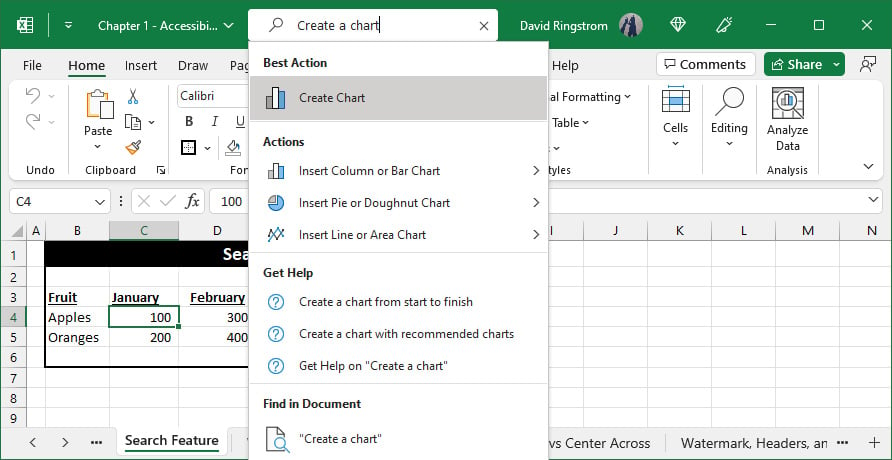
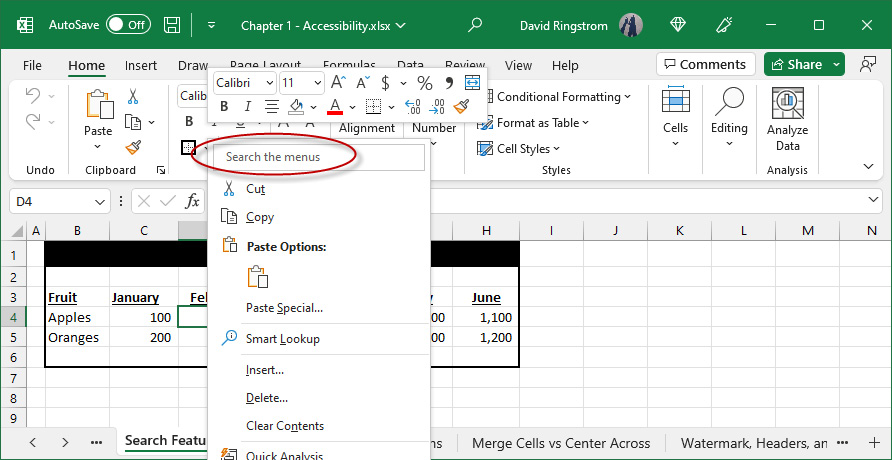
• Find in Document: Choose this option to search your document for the term or phrase that you entered. This is an alternative to choosing Home | Find & Select | Find or pressing Ctrl + F ( + F in Excel for macOS).
• Files: Recent workbooks you used that Excel determined may be relevant to the keyword or phrase that you entered.

The Microsoft Search box makes Excel more accessible, as it brings commands to you upon request. This turns the normal Excel experience on its head where users don’t remember where a command resides or whether a particular feature even exists.

Nuance

The Microsoft Search box is an effective means for finding commands in Excel, but it does a poor job with worksheet functions. The Insert Function command discussed earlier in this chapter is a more effective approach for unearthing functions. Further, not every command in the menu appears, even when you type it by name. For instance, typing Text to Columns shows alternatives but not the feature itself, which appears on the Data tab. Like many aspects of Excel, blind spots abound.

If you’re sensitive to changes in Excel’s user interface, you can collapse the Microsoft Search box down to an icon:

1. Choose File | Options | General.
2. Click Collapse the Microsoft Search box by default in the User Interface options section and then click OK.

A magnifying glass icon stays in place in the title bar, which you can click any time you wish to use the Microsoft Search box, or you can type Alt + Q in Excel for Windows. As shown in Figure 1.5, you can also access another version of the Microsoft Search box by right-clicking on any cell in Excel for Windows:

Figure 1.5 – Context menu-based search option

You can enter search terms into the context menu in the same fashion as the Microsoft Search box at the top of the screen. Now, let’s see how you can get more help in Excel.

Help tab of Excel’s Ribbon

The Help tab first appeared in Excel 2019 and is designed to provide immediate access to several support resources.

Figure 1.6 – Help tab

As shown in Figure 1.6, the Help tab of the Ribbon has the following commands:

• Help: Click this command or press F1 to display the Help task pane, which you can use to search for help on any aspect of Excel.

Nuance

Your device must be connected to the internet before you can use any command on the Help menu.

• Contact Support: This section requires you to enter a search term and then click Get Help. Relevant articles will appear, below which a Contact Support button enables you to create an online chat session with a Microsoft support agent. If you cancel the chat session, Microsoft will follow up with you via email.
• Feedback: This command enables you to send a smile to Microsoft for something you like about Excel, a frown for something you don’t like, or to send a suggestion.

Nuance

You may be surprised to learn that the Excel development team at Microsoft takes user feedback seriously. The Suggestion option enables you to not only suggest changes in Excel but also vote on requests by others. For instance, as of this writing, 276 votes were enough to get Microsoft to commit to adding Center Across Selection to the Home | Merge & Center drop-down menu. I’ll explain how to access Center Across Selection later in the Using Center Across Selection instead of merged cells section. The bottom line is, given the hundreds of millions of Excel users around the globe, it truly takes a handful of voices to effect change in Excel. If something is frustrating you about Excel, it’s probably bothered others as well, so take a moment to vote on someone else’s suggestion or post your own.

• Show Training: This command supplies instant access to a free video-based library of training materials that often includes downloadable templates so that you can follow along.
• What’s New: This command enables you to figure out whether any new features have been added to your version of Microsoft 365 recently.
• Community: This command links to a Microsoft-sanctioned online forum where you can ask and answer questions about Excel. Always be sure to search the forum before posting a new question because often you will find that your question has already been asked and answered.
• Excel Blog: This command opens a page with up-to-date news about Excel from the development team and is a straightforward way to keep up with new features that have been added recently or that are in development.

Let’s now look at ways to convert a list of data into an instant analysis.

On-demand PivotTables and charts

Excel offers three different approaches that allow any user to quickly transform a list of data into easy-to-understand reports or charts:

• Recommended PivotTables: This feature can create an instant report out of a list of data:
  1. Select any cell within the list on the World’s Longest Metro Systems worksheet of this chapter’s example workbook.
  2. Choose Insert | Recommended PivotTables.
  3. Choose any report from the Recommended PivotTables task pane shown in Figure 1.7:

Figure 1.7 – Recommended PivotTables task pane

Nuance

Recommended PivotTables appears as a dialog box in Excel 2021 and earlier. Your version of Microsoft 365 may still have the dialog box as well. New features are pushed out to users in waves, so there can be a delay of 6 months or more before the latest changes to Excel make it to your device.

Any reports that you generate by way of Recommended PivotTables are merely a starting point. You can add or remove fields as needed by way of the PivotTable Fields task pane, which appears when you click within any PivotTable.

• Recommended Charts: This artificial intelligence feature analyzes your data and makes suggestions as to which Excel charts are best suited to your needs:
  1. Select any cell within the list on the World’s Longest Metro Systems worksheet of this chapter’s example workbook.
  2. Click Insert | Recommended Charts.
  3. Choose a report from the Recommended Charts tab of the Insert Chart dialog box shown in Figure 1.8, and then click OK. In Excel for macOS, chart recommendations appear in a drop-down menu instead of a dialog box, and no rationale for why the chart is appropriate is offered.

Figure 1.8 – Recommended Charts dialog box

• Analyze Data: This feature can be thought of as Recommended Charts on steroids. The feature debuted as Insights and was renamed Ideas before being dubbed Analyze Data. You can not only create reports but also find unusual aspects within a list:
  1. Select any cell within the list on the World’s Longest Metro Systems worksheet of this chapter’s example workbook.
  2. Click Home | Analyze Data.
  3. Choose a report or chart from the Analyze Data task pane, or as shown in Figure 1.9, enter a plain English question such as stations per mile to create a chart that will show the distribution of stations by system length in miles. Depending upon the question you ask, Analyze Data will either create a chart, PivotChart, or PivotTable.

Figure 1.9 – Analyze Data task pane

Nuance

Presently, Analyze Data only works with datasets that have 1.5 million cells or less. The feature works best when your list is formatted as a Table, which I discuss how to do in Chapter 7, Automating Tasks with Tables. Dates in the yyyy-mm-dd format, such as 2024-01-01 for January 1, 2024, will be treated as text, although you can convert these to dates by using the DATEVALUE or VALUE functions, or by using the Text to Columns feature. To use this feature, select the dates that you wish to convert, choose Data | Text to Columns, click Next twice, choose Date, and then specify YMD from the corresponding list, and then click OK. Generally, the Text to Columns feature is used to separate a column of data into two or more columns, but it also works as a handy data transformation tool, especially when dates or numbers are formatted or stored as text.

Now that we’ve discussed some ways to make Excel more accessible, let’s see how to improve accessibility within individual workbooks.