We will be creating and accessing our MySQL databases by two different methods: by running our own independent Java programs and through a user interface tool named MySQL Workbench.

To download and install MySQL Workbench, go back to https://dev.mysql.com/downloads/ and select MySQL Workbench. Select your platform and click on the Download button. Then, run the installer.

In the window that comes up, drag the MsSQLWorkbench.app icon to the right, into the Applications folder:

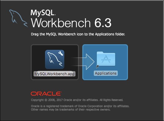
Figure A-14. Installing MySQL Workbench

After a few seconds, the app's icon will appear in the Applications folder. Launch it, and affirm that you want to open it:

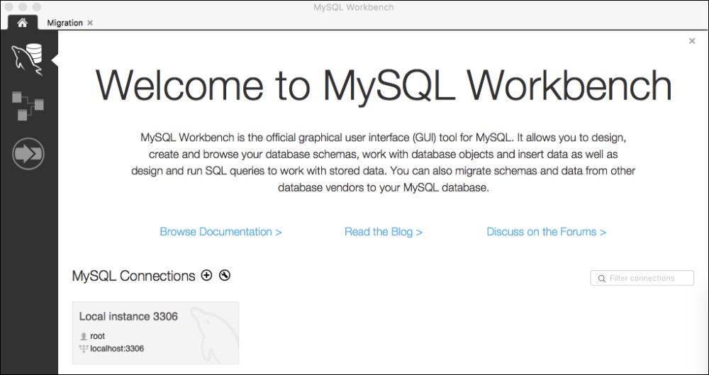
Figure A-15. Running the MySQL Workbench installer

Note that one connection is defined: localhost:3306 with the user root. The number 3306 is the port through which the connection is made.

Now that we have MySQL Workbench installed, we can test it. The main window for the app is shown in Figure A-16.

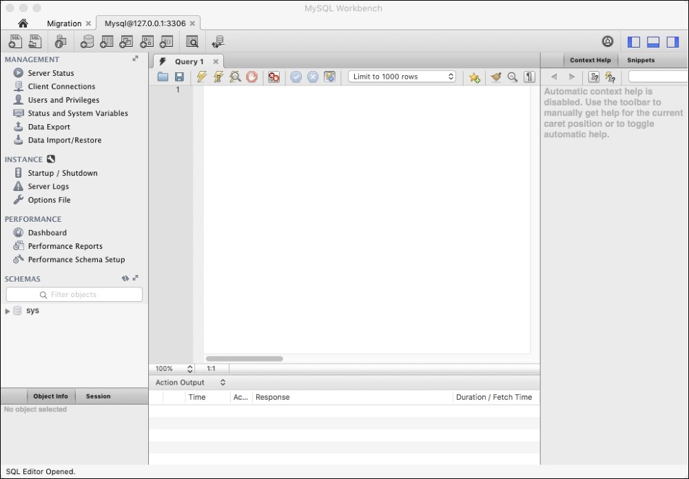
Figure A-16. The MySQL Workbench main window

Notice the tab labeled [email protected]:3306. That is the name of the connection that we have defined (here, 127.0.0.1 is the IP address of localhost). To actually connect to the database through that service, we must open the connection.

In the MySQL Workbench menu, select Database | Connect to Database.... Enter the password that you saved and click OK (see Figure A-17).

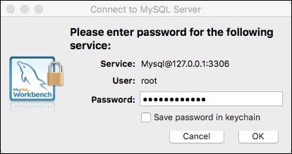
Figure A-17. Connecting to the MySQL Server

As soon as you get the chance, change your connection password to something simple and memorable.

Now your MySQL database is running and you have a live connection to it through this MySQLWorkbench interface (see Figure A-18).

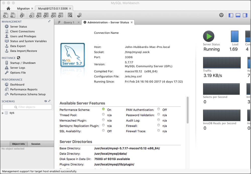
Figure A-18. The MySQL Workbench interface to the MySQL database

To create a database, click on this icon in the toolbar: This is the New Schema button. The image, which looks like a 55 gallon barrel of oil, is supposed to look like a big disk, representing a large amount of computer storage. It's a traditional representation of a database.

A new tabbed panel, labeled new_schema, opens. Technically, we are creating a schema on the MySQL Server.

Enter schema1 for Schema Name:

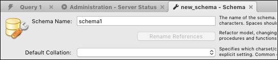
Figure A-19. Creating a database schema in MySQL

Then, click on the Apply button. Do the same on the Apply SQL Script to Database panel that pops up and then close that panel.

You now have two schemas listed under SCHEMAS in the sidebar: schema1 and sys. Double-click on schema1 to make it the current schema. That expands the listing to show its objects: Tables, Views, Stores Procedures, and Functions (see Figure A-20).

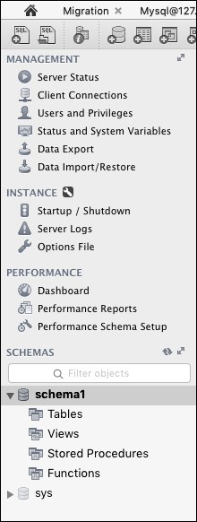
Figure A-20. schema1 objects

We can think of this as our current database. To add data to it, we must first create a table in it.

Click on the tab labeled Query 1 and then type the code shown in Figure A-21 into the editor.

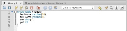
Figure A-21. SQL code

This is SQL code (SQL is the query language for RDBs). When this query is executed, it will create an empty database table named Friends that has four fields: lastName, firstName, sex, and yob. Notice that in SQL, the datatype is specified after the variable that it declares. The varchar type holds a variable-length character string of a length from 0 up to the specified limit (16 for lastName and 8 for firstName). The char type means a character string of exactly the specified length (1 for sex) and int stands for integer (whole number).

Note that SQL syntax requires a comma to separate each item in the declaration list, which is delimited by parentheses.

Also note that this editor (like the NetBeans editor) color-codes the syntax: blue for keywords (create, table, varchar, char, int) and orange for constants (16, 8, 1).

SQL is a very old computer language. When it was introduced in 1974, many keyboards still had only upper-case letters. So, it became customary to use all capital letters in SQL code. That tradition has carried over and many SQL programmers still prefer to type keywords in all caps, like this:

CREATE TABLE Friends (
    lastName VARCHAR(16),
    firstName VARCHAR(8),
    sex CHAR(1),
    yob INT
)

But it's really just a matter of style preference. The SQL interpreter accepts any combination of uppercase and lowercase letters for keywords.

To execute this query, click on the yellow lightning bolt on the tabbed panel's toolbar:

Expand the schema1 tree in the sidebar to confirm that your Friends table has been created as intended (see Figure A-22):

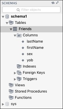
Figure A-22. Objects in schema1

Now we're ready to save some data about our friends.

Click on the new query button (or select File | New Query Tab). Then execute the query shown in Figure A-23. This adds one row (data point) to our Friends table. Notice that character strings are delimited by the apostrophe character, not quotation marks.

Next, execute the queries shown in Figure A-23, Figure A-24, and Figure A-25:

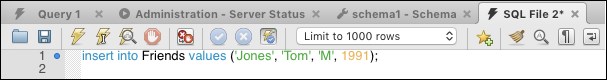
Figure A-23. An insertion

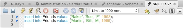
Figure A-24. Two more insertions

These add three rows (records) to the Friends table and then queries the table. The query is called a select statement. The asterisk (*) means to list all the rows of the table. The output is shown in the following Result Grid:

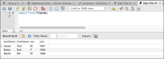
Figure A-25. A query