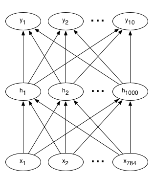
A typical neural network for a digit recognizer may have 784 input pixels connected to 1,000 neurons in the hidden layer, which in turn connects to 10 output targets — one for each digit. Each layer is fully connected to the layer above. A graphical representation of this network is shown as follows, where x are the inputs, h are the hidden neurons, and y are the output class variables:

In this notebook, we will build a neural network that will recognize handwritten numbers from 0-9.

The type of neural network that we are building is used in a number of real-world applications, such as recognizing phone numbers and sorting postal mail by address. To build this network, we will use the MNIST dataset.

We will begin as shown in the following code by importing all the required modules, after which the data will be loaded, and then finally building the network:

# Import Numpy, keras and MNIST data
import numpy as np
import matplotlib.pyplot as plt

from keras.datasets import mnist
from keras.models import Sequential
from keras.layers.core import Dense, Dropout, Activation
from keras.utils import np_utils

The MNIST dataset already comprises both training and test data. There are 60,000 data points of training data and 10,000 points of test data. If you do not have the data file locally at the '~/.keras/datasets/' + path, it can be downloaded at this location.

Each MNIST data point has:

• An image of a handwritten digit
• A corresponding label that is a number from 0-9 to help identify the image

The images will be called, and will be the input to our neural network, X; their corresponding labels are y.

We want our labels as one-hot vectors. One-hot vectors are vectors of many zeros and one. It's easiest to see this in an example. The number 0 is represented as [1, 0, 0, 0, 0, 0, 0, 0, 0, 0], and 4 is represented as [0, 0, 0, 0, 1, 0, 0, 0, 0, 0] as a one-hot vector.

We will use flattened data in this example, or a representation of MNIST images in one dimension rather than two can also be used. Thus, each 28 x 28 pixels number image will be represented as a 784 pixel 1 dimensional array.

By flattening the data, information about the 2D structure of the image is thrown; however, our data is simplified. With the help of this, all our training data can be contained in one array of shape (60,000, 784), wherein the first dimension represents the number of training images and the second depicts the number of pixels in each image. This kind of data is easy to analyze using a simple neural network, as follows:

# Retrieving the training and test data
(X_train, y_train), (X_test, y_test) = mnist.load_data()


print('X_train shape:', X_train.shape)
print('X_test shape: ', X_test.shape)
print('y_train shape:',y_train.shape)
print('y_test shape: ', y_test.shape)

The following function will help you visualize the MNIST data. By passing in the index of a training example, the show_digit function will display that training image along with its corresponding label in the title:

# Visualize the data
import matplotlib.pyplot as plt
%matplotlib inline

#Displaying a training image by its index in the MNIST set
def display_digit(index):
    label = y_train[index].argmax(axis=0)
    image = X_train[index]
    plt.title('Training data, index: %d,  Label: %d' % (index, label))
    plt.imshow(image, cmap='gray_r')
    plt.show()
    
# Displaying the first (index 0) training image
display_digit(0)
X_train = X_train.reshape(60000, 784)
X_test = X_test.reshape(10000, 784)
X_train = X_train.astype('float32')
X_test = X_test.astype('float32')
X_train /= 255
X_test /= 255
print("Train the matrix shape", X_train.shape)
print("Test the matrix shape", X_test.shape)


#One Hot encoding of labels.
from keras.utils.np_utils import to_categorical
print(y_train.shape)
y_train = to_categorical(y_train, 10)
y_test = to_categorical(y_test, 10)
print(y_train.shape)

For this example, you'll define the following:

• The input layer, which you should expect for each piece of MNIST data, as it tells the network the number of inputs
• Hidden layers, as they recognize patterns in data and also connect the input layer to the output layer
• The output layer, as it defines how the network learns and gives a label as the output for a given image, as follows:

# Defining the neural network
def build_model():
    model = Sequential()
    model.add(Dense(512, input_shape=(784,)))
    model.add(Activation('relu')) # An "activation" is just a non-linear function that is applied to the output
 # of the above layer. In this case, with a "rectified linear unit",
 # we perform clamping on all values below 0 to 0.
                           
    model.add(Dropout(0.2))   #With the help of Dropout helps we can protect the model from memorizing or "overfitting" the training data
    model.add(Dense(512))
    model.add(Activation('relu'))
    model.add(Dropout(0.2))
    model.add(Dense(10))
    model.add(Activation('softmax')) # This special "softmax" activation,
    #It also ensures that the output is a valid probability distribution,
    #Meaning that values obtained are all non-negative and sum up to 1.
    return model

#Building the model
model = build_model()
model.compile(optimizer='rmsprop',
          loss='categorical_crossentropy',
          metrics=['accuracy'])

Now that we've constructed the network, we feed it with data and train it, as follows:

# Training
model.fit(X_train, y_train, batch_size=128, nb_epoch=4, verbose=1,validation_data=(X_test, y_test))

After you're satisfied with the training output and accuracy, you can run the network on the test dataset to measure its performance!

A good result will obtain an accuracy higher than 95%. Some simple models have been known to achieve even up to 99.7% accuracy! We can test the model, as shown here:

# Comparing the labels predicted by our model with the actual labels

score = model.evaluate(X_test, y_test, batch_size=32, verbose=1,sample_weight=None)
# Printing the result
print('Test score:', score[0])
print('Test accuracy:', score[1])