Introduction to R packages – rattle

Before discussing one or two examples of using rattle, it might be a good idea to discuss an R package called rattle.data. As its name suggests, we could guess that it contains data used by rattle. It is a good idea to use a small dataset to generate a dendrogram. For the next case, we use the first 20 observations from a dataset called wine:

library(rattle.data) 
data(wine)  
x<-head(wine,20) 

To launch rattle, we have the following two lines:

library(rattle) 
rattle() 

For data, we choose R Dataset, then choose x, as shown in the following screenshot. To save space, only the top part is presented here:

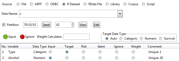
The following screenshot shows our choice:

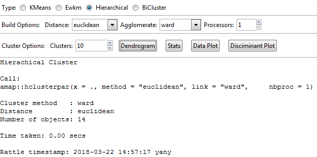
From the previous screenshot, we see 14 observations. Click Clusters, with a default of 10 clusters, and Dendrogram. See the result in the following screenshot:

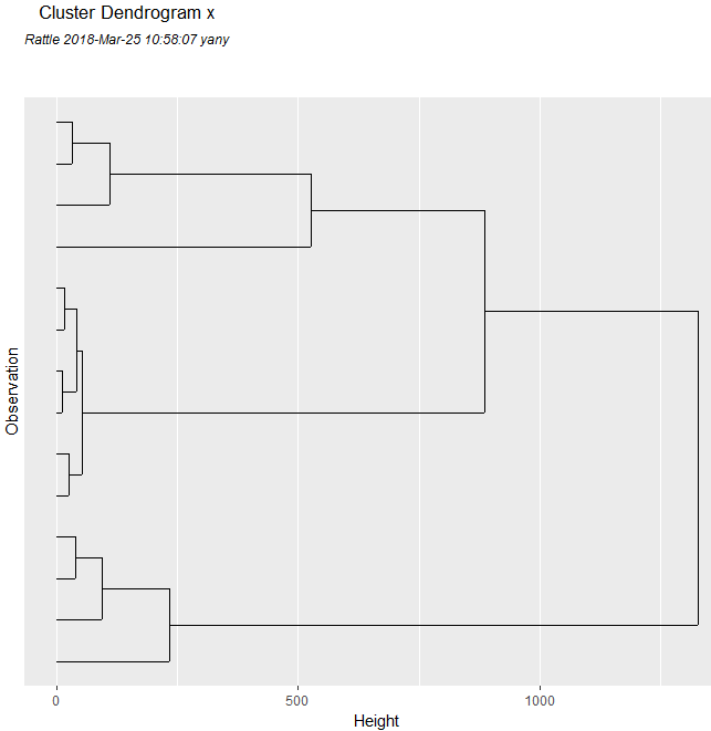
The previous dendrogram...