DMVs and DMFs

In this section, we will show you several dynamic management views (DMVs) and dynamic management functions (DMFs) that can help you to find out the number of server resources that are being used by your queries and to find the most expensive queries in your SQL Server instance.

sys.dm_exec_requests and sys.dm_exec_sessions

The sys.dm_exec_requests DMV can be used to display the requests currently executing on SQL Server, whereas sys.dm_exec_sessions shows the authenticated sessions on the instance. Although these DMVs include many columns, in this section, we will focus on the ones related to resource usage and query performance. You can look at the definitions of the other columns on the SQL Server documentation.

Both DMVs share several columns, as shown in the following table:

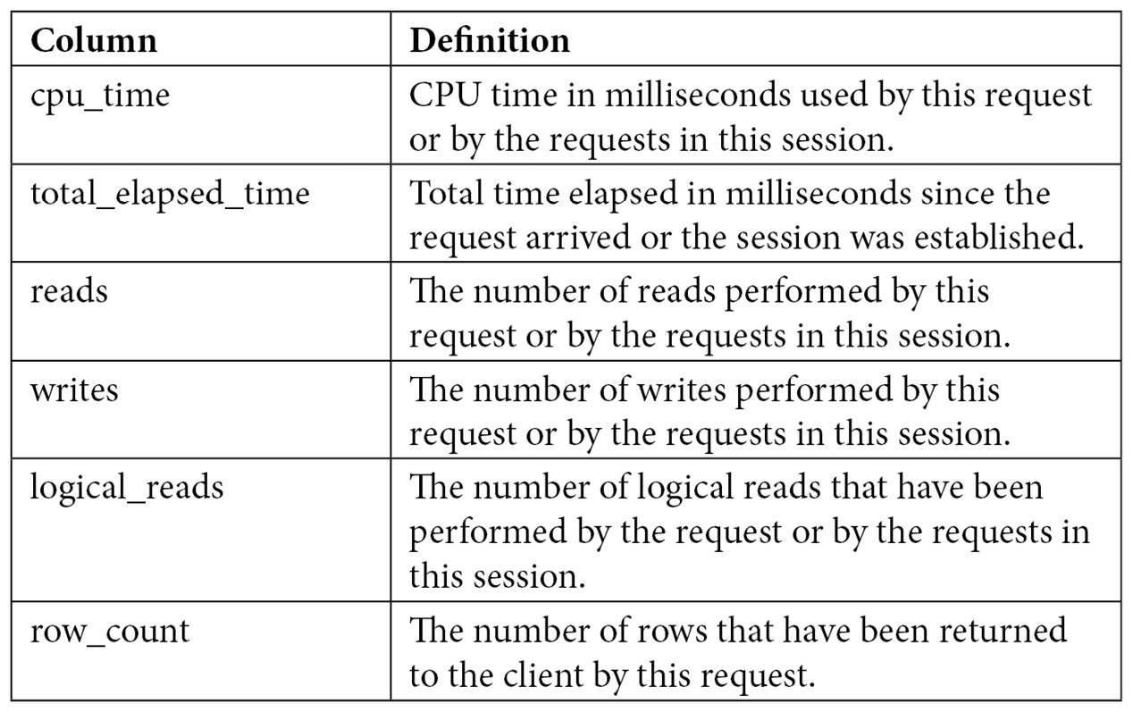
Table 2.1 – The sys.dm_exec_requests and sys.dm_exec_sessions columns

sys.dm_exec_requests will show the resources that are used by a specific request currently executing, whereas sys.dm_exec_sessions will show the accumulated resources of all the requests completed by a session. To understand how these two DMVs collect resource usage information, we can use a query that takes at least a few seconds. Open a new query in Management Studio and get its session ID (for example, using SELECT @@SPID), but make sure you don’t run anything on it yet – the resource usage will be accumulated on the sys.dm_exec_sessions DMV. Copy and be ready to run the following code on that window:

DBCC FREEPROCCACHE
DBCC DROPCLEANBUFFERS
GO
SELECT * FROM Production.Product p1 CROSS JOIN Production.Product p2

Copy the following code to a second window, replacing session_id with the value you obtained in the first window:

SELECT cpu_time, reads, total_elapsed_time, logical_reads, row_count
FROM sys.dm_exec_requests
WHERE session_id = 56
GO
SELECT cpu_time, reads, total_elapsed_time, logical_reads, row_count
FROM sys.dm_exec_sessions
WHERE session_id = 56

Run the query on the first session and, at the same time, run the code on the second session several times to see the resources used. The following output shows a sample execution while the query is still running and has not been completed yet. Notice that the sys.dm_exec_requests DMV shows the partially used resources and that sys.dm_exec_sessions shows no used resources yet. Most likely, you will not see the same results for sys.dm_exec_requests:

After the query completes, the original request no longer exists and sys.dm_exec_requests returns no data at all. sys.dm_exec_sessions now records the resources used by the first query:

If you run the query on the first session again, sys.dm_exec_sessions will accumulate the resources used by both executions, so the values of the results will be slightly more than twice their previous values, as shown here:

Keep in mind that CPU time and duration may vary slightly during different executions and that you will likely get different values as well. The number of reads for this execution is 8,192, and we can see the accumulated value of 16,384 for two executions. In addition, the sys.dm_exec_requests DMV only shows information of currently executing queries, so you may not see this particular data if a query completes before you can query it.

In summary, sys.dm_exec_requests and sys.dm_exec_sessions are useful for inspecting the resources being used by a request or the accumulation of resources being used by requests on a session since its creation.

Sys.dm_exec_query_stats

If you’ve ever worked with any version of SQL Server older than SQL Server 2005, you may remember how difficult it was to find the most expensive queries in your instance. Performing that kind of analysis usually required running a server trace in your instance for some time and then analyzing the collected data, usually in the size of gigabytes, using third-party tools or your own created methods (a very time-consuming process). Not to mention the fact that running such a trace could also affect the performance of a system, which most likely is having a performance problem already.

DMVs were introduced with SQL Server 2005 and are a great help to diagnose problems, tune performance, and monitor the health of a server instance. In particular, sys.dm_exec_query_stats provides a rich amount of information not available before in SQL Server regarding aggregated performance statistics for cached query plans. This information helps you avoid the need to run a trace, as mentioned earlier, in most cases. This view returns a row for each statement available in the plan cache, and SQL Server 2008 added enhancements such as the query hash and plan hash values, which will be explained shortly.

Let’s take a quick look at understanding how sys.dm_exec_query_stats works and the information it provides. Create the following stored procedure with three simple queries:

CREATE PROC test
AS
SELECT * FROM Sales.SalesOrderDetail WHERE SalesOrderID = 60677
SELECT * FROM Person.Address WHERE AddressID = 21
SELECT * FROM HumanResources.Employee WHERE BusinessEntityID = 229

Run the following code to clean the plan cache (so that it is easier to inspect), remove all the clean buffers from the buffer pool, execute the created test stored procedure, and inspect the plan cache. Note that the code uses the sys.dm_exec_sql_text DMF, which requires a sql_handle or plan_handle value and returns the text of the SQL batch:

DBCC FREEPROCCACHE
DBCC DROPCLEANBUFFERS
GO
EXEC test
GO
SELECT * FROM sys.dm_exec_query_stats
CROSS APPLY sys.dm_exec_sql_text(sql_handle)
WHERE objectid = OBJECT_ID('dbo.test')

Examine the output. Because the number of columns is too large to show in this book, only some of the columns are shown here:

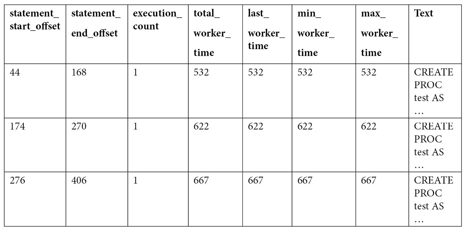
As you can see by looking at the query text, all three queries were compiled as part of the same batch, which we can also verify by validating they have the same plan_handle and sql_handle. statement_start_offset and statement_end_offset can be used to identify the particular queries in the batch, a process that will be explained later in this section. You can also see the number of times the query was executed and several columns showing the CPU time used by each query, such as total_worker_time, last_worker_time, min_worker_time, and max_worker_time. Should the query be executed more than once, the statistics would show the accumulated CPU time on total_worker_time. Not shown in the previous output are additional performance statistics for physical reads, logical writes, logical reads, CLR time, and elapsed time. The following table shows the list of columns, including performance statistics and their documented description:

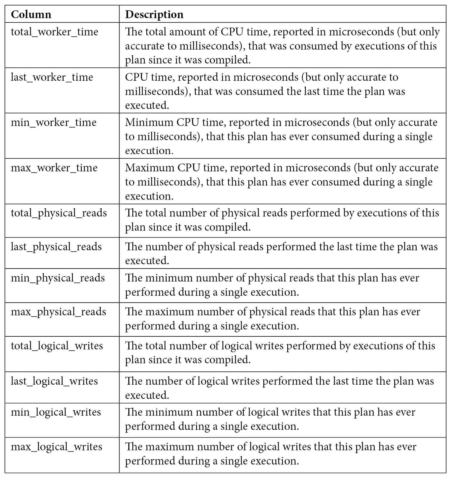
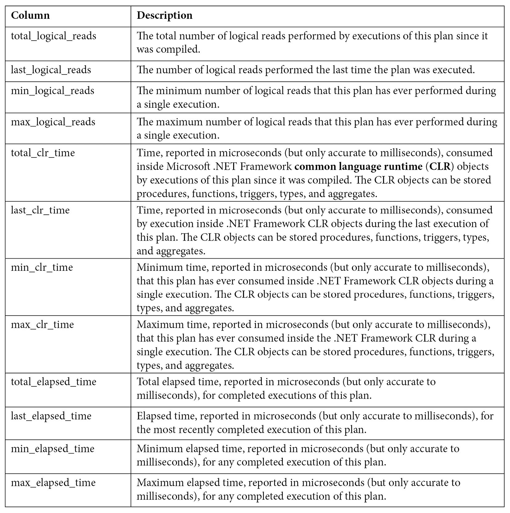
Table 2.2 – The sys.dm_exec_query_stats columns

Keep in mind that this view only shows statistics for completed query executions. You can look at sys.dm_exec_requests, as explained earlier, for information about queries currently executing. Finally, as explained in the previous chapter, certain types of execution plans may never be cached, and some cached plans may also be removed from the plan cache for several reasons, including internal or external memory pressure on the plan cache. Information for these plans will not be available on sys.dm_exec_query_stats.

Now, let’s look at the statement_start_offset and statement_end_offset values.

Understanding statement_start_offset and statement_end_offset

As shown from the previous output of sys.dm_exec_query_stats, the sql_handle, plan_handle, and text columns showing the code for the stored procedure are the same in all three records. The same plan and query are used for the entire batch. So, how do we identify each of the SQL statements, for example, supposing that only one of them is expensive? We must use the statement_start_offset and statement_end_offset columns. statement_start_offset is defined as the starting position of the query that the row describes within the text of its batch, whereas statement_end_offset is the ending position of the query that the row describes within the text of its batch. Both statement_start_offset and statement_end_offset are indicated in bytes, starting with 0. A value of –1 indicates the end of the batch.

We can easily extend our previous query to inspect the plan cache to use statement_start_offset and statement_end_offset and get something like the following:

DBCC FREEPROCCACHE
DBCC DROPCLEANBUFFERS
GO
EXEC test
GO
SELECT SUBSTRING(text, (statement_start_offset/2) + 1,
((CASE statement_end_offset
WHEN -1
THEN DATALENGTH(text)
ELSE
statement_end_offset
END
- statement_start_offset)/2) + 1) AS statement_text, *
FROM sys.dm_exec_query_stats
CROSS APPLY sys.dm_exec_sql_text(sql_handle)
WHERE objectid = OBJECT_ID('dbo.test')

This would produce output similar to the following (only a few columns are shown here):

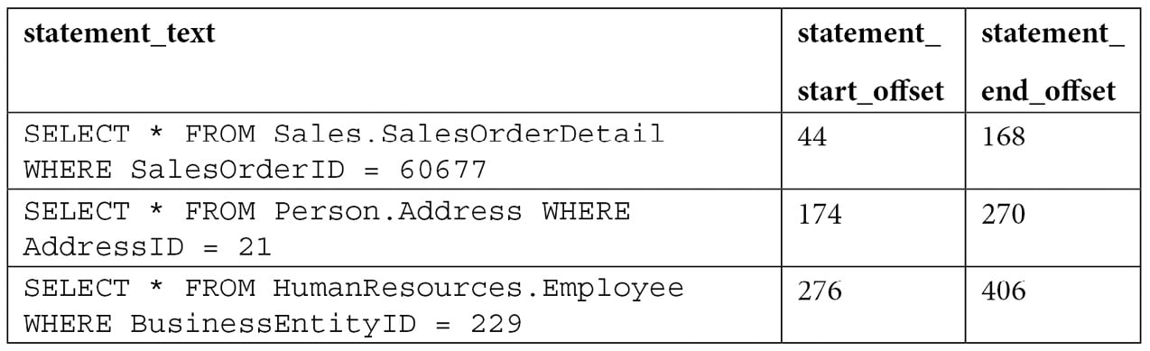
The query makes use of the SUBSTRING function, as well as statement_start_offset and statement_end_offset values, to obtain the text of the query within the batch. Division by 2 is required because the text data is stored as Unicode.

To test the concept for a particular query, you can replace the values for statement_start_offset and statement_end_offset directly for the first statement (44 and 168, respectively) and provide sql_handle or plan_handle, (returned in the previous query and not printed in the book) as shown here, to get the first statement that was returned:

SELECT SUBSTRING(text, 44 / 2 + 1, (168 - 44) / 2 + 1) FROM sys.dm_exec_sql_text(0x03000500996DB224E0B27201B7A1000001000000000000 000000000000000000000000000000000000000000)

sql_handle and plan_handle

The sql_handle value is a hash value that refers to the batch or stored procedure the query is part of. It can be used in the sys.dm_exec_sql_text DMF to retrieve the text of the query, as demonstrated previously. Let’s use the example we used previously:

SELECT * from sys.dm_exec_sql_text(0x03000500996DB224E0B27201B7A1000001000000 000000000000000000000000000000000000000000000000)

We would get the following in return:

The sql_handle hash is guaranteed to be unique for every batch in the system. The text of the batch is stored in the SQL Manager Cache or SQLMGR, which you can inspect by running the following query:

SELECT * FROM sys.dm_os_memory_objects
WHERE type = 'MEMOBJ_SQLMGR'

Because a sql_handle has a 1:N relationship with a plan_handle (that is, there can be more than one generated executed plan for a particular query), the text of the batch will remain on the SQLMGR cache store until the last of the generated plans is evicted from the plan cache.

The plan_handle value is a hash value that refers to the execution plan the query is part of and can be used in the sys.dm_exec_query_plan DMF to retrieve such an execution plan. It is guaranteed to be unique for every batch in the system and will remain the same, even if one or more statements in the batch are recompiled. Here is an example:

SELECT * FROM sys.dm_exec_query_plan(0x05000500996DB224B0C9B8F8010000000100 0000000000000000000000000000000000000000000000000000)

Running the preceding code will return the following output, and clicking the query_plan link will display the requested graphical execution plan. Again, make sure you are using a valid plan_handle value:

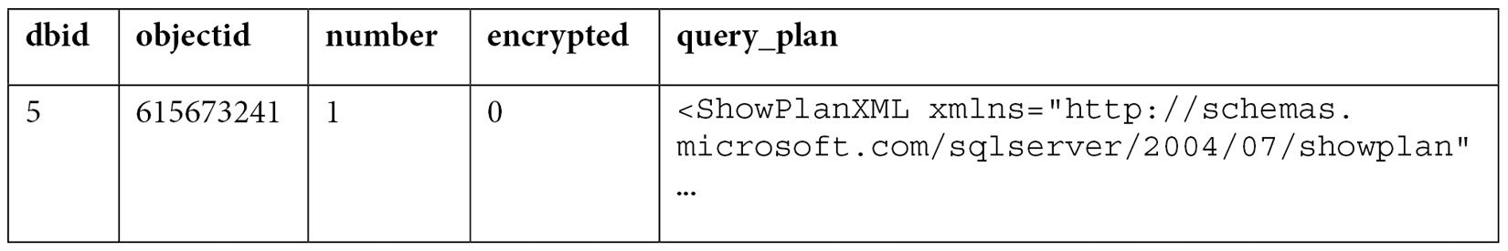
Cached execution plans are stored in the SQLCP and OBJCP cache stores: object plans, including stored procedures, triggers, and functions, are stored in the OBJCP cache store, whereas plans for ad hoc, auto parameterized, and prepared queries are stored in the SQLCP cache store.

query_hash and plan_hash

Although sys.dm_exec_query_stats was a great resource that provided performance statistics for cached query plans when it was introduced in SQL Server 2005, one of its limitations was that it was not easy to aggregate the information for the same query when this query was not parameterized. The query_hash and plan_hash columns, introduced with SQL Server 2008, provide a solution to this problem. To understand the problem, let’s look at an example of the behavior of sys.dm_exec_query_stats when a query is auto-parameterized:

DBCC FREEPROCCACHE
DBCC DROPCLEANBUFFERS
GO
SELECT * FROM Person.Address
WHERE AddressID = 12
GO
SELECT * FROM Person.Address
WHERE AddressID = 37
GO
SELECT * FROM sys.dm_exec_query_stats

Because AddressID is part of a unique index, the AddressID = 12 predicate would always return a maximum of one record, so it is safe for the query optimizer to auto-parameterize the query and use the same plan. Here is the output:

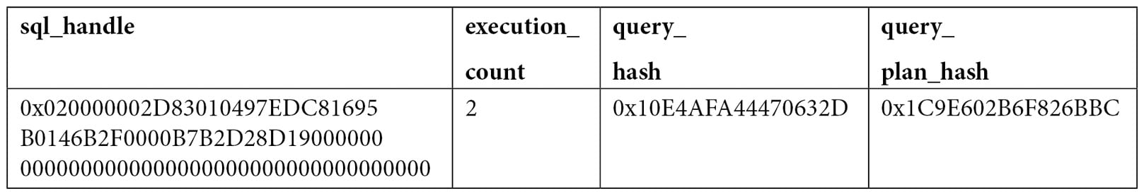
In this case, we only have one plan that’s been reused for the second execution, as shown in the execution_count value. Therefore, we can also see that plan reuse is another benefit of parameterized queries. However, we can see a different behavior by running the following query:

DBCC FREEPROCCACHE
DBCC DROPCLEANBUFFERS
GO
SELECT * FROM Person.Address
WHERE StateProvinceID = 79
GO
SELECT * FROM Person.Address
WHERE StateProvinceID = 59
GO
SELECT * FROM sys.dm_exec_query_stats

Because a filter with an equality comparison on StateProvinceID could return zero, one, or more values, it is not considered safe for SQL Server to auto-parameterize the query; in fact, both executions return different execution plans. Here is the output:

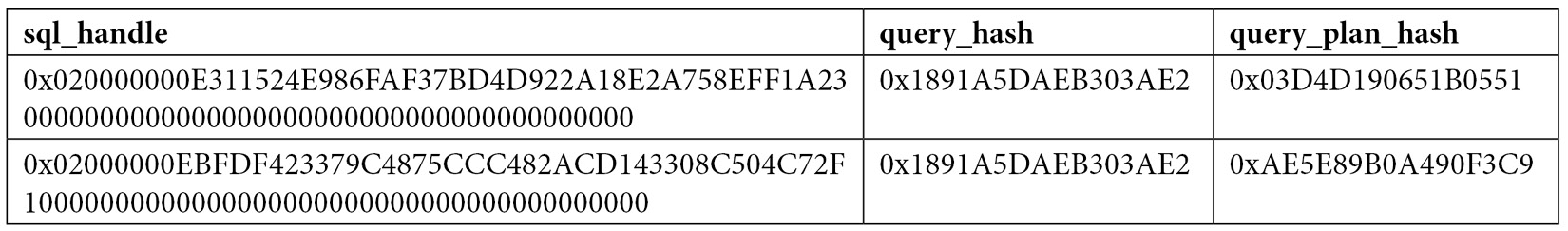
As you can see, sql_handle, plan_handle (not shown), and query_plan_hash have different values because the generated plans are different. However, query_hash is the same because it is the same query, only with a different parameter. Supposing that this was the most expensive query in the system and there are multiple executions with different parameters, it would be very difficult to find out that all those execution plans do belong to the same query. This is where query_hash can help. You can use query_hash to aggregate performance statistics of similar queries that are not explicitly or implicitly parameterized. Both query_hash and plan_hash are available on the sys.dm_exec_query_stats and sys.dm_exec_requests DMVs.

The query_hash value is calculated from the tree of logical operators that was created after parsing just before query optimization. This logical tree is used as the input to the query optimizer. Because of this, two or more queries do not need to have the same text to produce the same query_hash value since parameters, comments, and some other minor differences are not considered. And, as shown in the first example, two queries with the same query_hash value can have different execution plans (that is, different query_plan_hash values). On the other hand, query_plan_hash is calculated from the tree of physical operators that makes up an execution plan. If two plans are the same, although very minor differences are not considered, they will produce the same plan hash value as well.

Finally, a limitation of the hashing algorithms is that they can cause collisions, but the probability of this happening is extremely low. This means that two similar queries may produce different query_hash values or that two different queries may produce the same query_hash value, but again, the probability of this happening is extremely low, and it should not be a concern.

Finding expensive queries

Now, let’s apply some of the concepts explained in this section and use the sys.dm_exec_query_stats DMV to find the most expensive queries in your system. A typical query to find the most expensive queries on the plan cache based on CPU is shown in the following code. Note that the query is grouped on the query_hash value to aggregate similar queries, regardless of whether or not they are parameterized:

SELECT TOP 20 query_stats.query_hash,
SUM(query_stats.total_worker_time) / SUM(query_stats.execution_count)
AS avg_cpu_time,
MIN(query_stats.statement_text) AS statement_text
FROM
(SELECT qs.*,
SUBSTRING(st.text, (qs.statement_start_offset/2) + 1,
 ((CASE statement_end_offset
WHEN -1 THEN DATALENGTH(ST.text)
ELSE qs.statement_end_offset END
- qs.statement_start_offset)/2) + 1) AS statement_text
FROM sys.dm_exec_query_stats qs
CROSS APPLY sys.dm_exec_sql_text(qs.sql_handle) AS st) AS query_stats
GROUP BY query_stats.query_hash
ORDER BY avg_cpu_time DESC

You may also notice that each returned row represents a query in a batch (for example, a batch with five queries would have five records on the sys.dm_exec_query_stats DMV, as explained earlier). We could trim the previous query into something like the following query to focus on the batch and plan level instead. Notice that there is no need to use the statement_start_offset and statement_end_offset columns to separate the particular queries and that this time, we are grouping on the query_plan_hash value:

SELECT TOP 20 query_plan_hash,
SUM(total_worker_time) / SUM(execution_count) AS avg_cpu_time,
MIN(plan_handle) AS plan_handle, MIN(text) AS query_text
FROM sys.dm_exec_query_stats qs
CROSS APPLY sys.dm_exec_sql_text(qs.plan_handle) AS st
GROUP BY query_plan_hash
ORDER BY avg_cpu_time DESC

These examples are based on CPU time (worker time). Therefore, in the same way, you can update these queries to look for other resources listed on sys.dm_exec_query_stats, such as physical reads, logical writes, logical reads, CLR time, and elapsed time.

Finally, we could also apply the same concept to find the most expensive queries that are currently executing, based on sys.dm_exec_requests, as shown in the following query:

SELECT TOP 20 SUBSTRING(st.text, (er.statement_start_offset/2) + 1,
((CASE statement_end_offset
WHEN -1
THEN DATALENGTH(st.text)
ELSE
er.statement_end_offset
END
- er.statement_start_offset)/2) + 1) AS statement_text
, *
FROM sys.dm_exec_requests er
CROSS APPLY sys.dm_exec_sql_text(er.sql_handle) st
ORDER BY total_elapsed_time DESC

Blocking and waits

We have talked about queries using resources such as CPU, memory, or disk and measured as CPU time, logical reads, and physical reads, among other performance counters. In SQL Server, however, those resources may not available immediately and your queries may have to wait until they are, causing delays and other performance problems. Although those waits are expected and could be unnoticeable, in some cases, this could be unacceptable, requiring additional troubleshooting. SQL Server provides several ways to track these waits, including several DMVs, which we will cover next, or the WaitsStat element, which we covered in Chapter 1, An Introduction to Query Tuning and Optimization.

Blocking can be seen as a type of wait and occurs all the time on relational databases, as it is required for applications to correctly access and change data. But its duration should be unnoticeable and should not impact applications. So, similar to most other wait types, excessive blocking could be a common performance problem too.

Finally, there are some wait types that, even in large wait times, never impact the performance of some other queries. A few examples of such wait types are LAZYWRITER_SLEEP, LOGMGR_QUEUE, and DIRTY_PAGE_POOL and they are typically filtered out when collecting wait information.

Let me show you a very simple example of blocking so that you can understand how to detect it and troubleshoot it. Using the default isolation level, which is read committed, the following code will block any operation trying to access the same data:

BEGIN TRANSACTION
UPDATE Sales.SalesOrderHeader
SET Status = 1
WHERE SalesOrderID = 43659

If you open a second window and run the following query, it will be blocked until the UPDATE transaction is either committed or rolled back:

SELECT * FROM Sales.SalesOrderHeader

Two very simple ways to see if blocking is the problem, and to get more information about it, is to run any of the following queries. The first uses the traditional but now deprecated catalog view – that is, sysprocesses:

SELECT * FROM sysprocesses
WHERE blocked <> 0

The second method uses the sys.dm_exec_requests DMV, as follows:

SELECT * FROM sys.dm_exec_requests
WHERE blocking_session_id <> 0

In both cases, the blocked or blocking_session_id columns will show the session ID of the blocking process. They will also provide information about the wait type, which in this case is LCK_M_S, the wait resource, which in this case is the data page number (10:1:16660), and the waiting time so far in milliseconds. LCK_M_S is only one of the multiple lock modes available in SQL Server.

Notice that in the preceding example, sysprocesses and sys.dm_requests only return the row for the blocked process, but you can use the same catalog view and DMV, respectively, to get additional information about the blocking process.

An additional way to find the blocking statement could be to use the DBCC INPUTBUFFER statement or the sys.dm_exec_input_buffer DMF and prove it with the blocking session ID. This can be seen here:

SELECT * FROM sys.dm_exec_input_buffer(70, 0)

Finally, roll back the current transaction to cancel the current UPDATE statement:

ROLLBACK TRANSACTION

Let’s extend our previous example to show a CXPACKET and other waits but this time while blocking the first record of SalesOrderDetail. We need a bigger table to encourage a parallel plan:

BEGIN TRANSACTION
UPDATE Sales.SalesOrderDetail
SET OrderQty = 3
WHERE SalesOrderDetailID = 1

Now, open a second query window and run the following query. Optionally, request an actual execution plan:

SELECT * FROM Sales.SalesOrderDetail
ORDER BY OrderQty

Now, open yet another query window and run the following, replacing 63 with the session ID from running your SELECT statement:

SELECT * FROM sys.dm_os_waiting_tasks
WHERE session_id = 63

This time, you may see a row per session ID and execution context ID. In my test, there is only one process waiting on LCK_M_S, as in our previous example, plus eight context IDs waiting on CXPACKET waits.

Complete this exercise by canceling the transaction again:

ROLLBACK TRANSACTION

You can also examine the execution plan, as covered in the previous chapter, to see the wait information, as shown in the following plan extract. My plan returned eight wait types, four of which are shown here:

<WaitStats>
    <Wait WaitType="CXPACKET" WaitTimeMs="2004169" WaitCount="1745" />
    <Wait WaitType="LCK_M_S" WaitTimeMs="249712" WaitCount="1" />
    <Wait WaitType="ASYNC_NETWORK_IO" WaitTimeMs="746" WaitCount="997" />
    <Wait WaitType="LATCH_SH" WaitTimeMs="110" WaitCount="5" />
…
</WaitStats>

Blocking and waits could be more complicated topics. For more details, please refer to the SQL Server documentation.

Now that we have covered DMVs and DMFs, it is time to explore SQL Trace, which can also be used to troubleshoot queries in SQL Server.