
Integers, bits, bytes, and Booleans
While Julia is usually dynamically typed—that is, in common with most interpreted languages, it does not require the type to be specified when a variable is declared; rather, it infers it from the form of the declaration. However, it also can be considered as a strongly typed language and, in this case, allows the programmer to specify a variable’s type precisely.
A variable in Julia is any combination of upper- or lowercase letters, digits, and the underscore (_) and exclamation (!) characters. It must start with a letter or an underscore.
Conventionally, variable names consist of lowercase letters with long names separated by underscores rather than using camel case.
To determine a variable type, we can use the typeof() function, as follows:
julia>x = 2; typeof(x) # => gives Intjulia>x = 2.0; typeof(x) # => gives Float
Notice that the type (see the preceding code) starts with a capital letter and ends with a number, which indicates the number of bit length of the variable. The bit length defaults to the word length of the operating system, and this can be determined by examining the WORD_SIZE built-in constant, as follows:
julia> WORD_SIZE # => 64 (on my MacPro computer)In this section, we will be dealing first with integer and Boolean types.
Integers
An integer type can be any of Int8, Int16, Int32, Int64, and Int128, so the maximum integer can occupy 16 bytes of storage and be anywhere within the range of –2127 to (+2127 - 1).
If we need more precision than this, Julia core implements the BigInt type:
julia> x = BigInt(2^32)
6277101735386680763835789423207666416102355444464034512896
As well as the integer type, Julia provides the unsigned integer type, UInt; again, UInt ranges from 8 to 128 bytes, so the maximum UInt value is (2128 - 1).
We can use the typemax() and typemax() functions to output the ranges of the Int and UInt types, like so:
julia> for T =
  Any[Int8,Int16,Int32,Int64,Int128,UInt8,UInt16,UInt32,UInt64,UInt128]
  println("$(lpad(T,7)): [$(typemin(T)),$(typemax(T))]")
end
Int8: [-128,127]
Int16: [-32768,32767]
Int32: [-2147483648,2147483647]
Int64: [-9223372036854775808,9223372036854775807]
Int128: [-170141183460469231731687303715884105728,
          170141183460469231731687303715884105727]
UInt8: [0, 255]
UInt16: [0, 65535]
UInt32: [0, 4294967295]
UInt64: [0, 18446744073709551615]
UInt128: [0, 340282366920938463463374607431768211455]
Particularly, notice the use of the form of the for statement, which we will discuss when we deal with arrays and matrices later in this chapter.
Suppose we type the following:
julia> x = 2^32; x*x # => the answer 0The reason for the answer being 0 is that the integer “wraps” around, so squaring 232 gives 0, not 264, since my WORD_SIZE value is 64:
julia> x = int128(2^32); x*x
# => the answer we would expect 18446744073709551616
We can use the typeof() function on a type such as Int64 in order to see what its parent type is:
# So typeof(Int64) gives DataType and typeof(UInt128) also gives DataType.
A definition of DataType is hinted at in the boot.jl core file; I say hinted at because the actual definition is implemented in C, and the Julia equivalent is commented out.
Definitions of the integer types can also be found in boot.jl, this time not commented out.
In the next chapter, we will discuss the Julia type system in some detail. Here, it is worth noting that we distinguish between two kinds of data types: abstract and primitive (concrete).
The general syntax for declaring an abstract type is shown here:
abstract type «name» end
abstract type «name» <: «supertype» end
Typically, this is how it would look:
abstract type Number end
abstract type Real <: Number end
abstract type AbstractFloat <: Real end
abstract type Integer <: Real end
abstract type Signed <: Integer end
abstract type Unsigned <: Integer end
Here, the <: operator corresponds to a subclass of the parent.
Let’s suppose we type the following:
julia> x = 7; y = 5; x/y # => this gives 1.4Here, the division of two integers produces a real result. In interactive mode, we can use the ans symbol to correspond to the last answer—that is, typeof(ans) gives Float.
To get the integer divisor, we use the div(x,y) function, which gives 1, as expected, and typeof(ans) is Int64. The remainder is obtained either by rem(x,y) or by using the % operator.
Julia has one curious operator—the backslash. Syntactically, x\y is equivalent to y/x. So, with x and y, as before, x\y gives 0.71428 (to 5 decimal places).
Primitive types
A primitive type is a concrete type whose data consists of a series of bits. Examples of primitive types are the (well-known) integers and floating-point values that we have met previously.
The general syntax for declaring a primitive type is like that of an abstract type but with the addition of the number of bits to be allocated:
primitive type «name» «bits» end
primitive type «name» <: «supertype» «bits» end
Since Julia is written (mostly) in Julia, a corollary is that Julia lets you declare your own primitive types, rather than providing only a fixed set of built-in ones.
That is, all the standard primitive types are defined in Base itself, as follows:
primitive type Float16 <: AbstractFloat 16 end
primitive type Float32 <: AbstractFloat 32 end
primitive type Float64 <: AbstractFloat 64 end
primitive type Bool <: Integer 8 end
primitive type Char 32 end
primitive type Int8 <: Signed 8 end
primitive type UInt8 <: Unsigned 8 end
primitive type Int16 <: Signed 16 end
primitive type UInt16 <: Unsigned 16 end
primitive type Int32 <: Signed 32 end
primitive type UInt32 <: Unsigned 32 end
primitive type Int64 <: Signed 64 end
primitive type UInt64 <: Unsigned 64 end
primitive type Int128 <: Signed 128 end
primitive type UInt128 <: Unsigned 128 end
Note that only sizes that are multiples of 8 bits are supported, so Boolean values, although they really need just a single bit, cannot be declared to be any smaller than 8 bits. Figure 2.1 demonstrates a portion of the Julia hierarchical structure as it applies to simple numerical types:
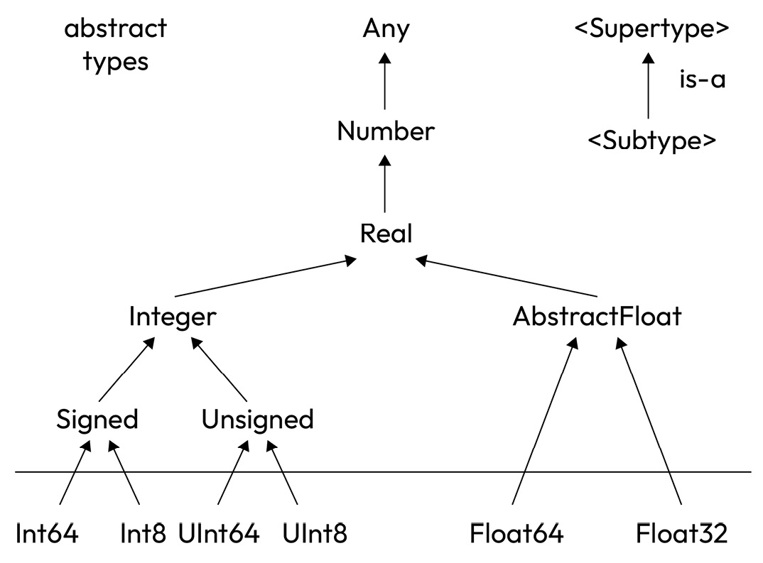
Figure 2.1 – Tree structure for numerical types
Those above the line are abstract types beginning with Any and cascading down through Number and Real before splitting into Integer and AbstractFloat types, eventually reaching the primitive types defined in Julia Base, which are shown below the line.
Primitives can’t be subclassed further, hence terminating the various branches of the tree.
Logical and arithmetic operators
As well as decimal arguments it is possible to assign binary, octal, and hexadecimal ones using the 0b, 0o, and 0x prefixes.
So, x = 0b110101 creates the hexadecimal number 0x35 (that is, decimal 53), and typeof(ans) is UInt8 since 53 will “fit” into a single byte.
For larger values, the type is correspondingly higher—that is, x = 0b1000010110101 gives x = 0x10b5, and typeof(ans) is UInt.
When operating on bits, Julia provides ~ (not), | (or), & (and), and $ (xor):
julia>x = 0xbb31; y = 0xaa5f;julia>x$y 0x116e
Also, we can perform arithmetic shifts using the (LEFT) and (RIGHT) operators.
Note
Because x is of the UInt16 type, the shift operator retains that size, so x = 0xbb31; x<<8. This gives 0x3100 (the top two nibbles being discarded), and typeof(ans) is UInt.
Booleans
Julia has the Bool logical type. Dynamically, a variable is assigned a Bool type by equating it to the true or false constant (both lowercase), or alternatively, to a logical expression such as the following:
julia>p = (2 < 3) # => truejulia>typeof(p) # => Bool
Many languages treat 0, empty strings, and NULL instances as representing false and anything else as true. This is NOT the case in Julia, however; there are cases where a Bool value may be promoted to an integer, in which case true corresponds to unity.
That is, an expression such as x + p (where x is of the Int type and p of the Bool type) will output the following:
julia>x = 0xbb31; p = (2 < 3);julia>x + p 0xbb32julia>typeof(ans) # => UInt16
Big integers
Let’s consider the factorial function defined by the usual recursive relation:
# n! = n*(n-1)! for integer values of n (> 0)
function fac(n::Integer)
  @assert n > 0
  (n == 1) ? 1 : n*fac(n-1)
end
Note that since normally, integers in Julia overflow (a feature of Low-Level Virtual Machine (LLVM), the preceding definition can lead to problems with large values of n, as illustrated here:
julia>using Printf for i = 20:30 @printf "%3d : %d\n" i fac(i) end 20 : 2432902008176640000 21 : -4249290049419214848 22 : -1250660718674968576 23 : 8128291617894825984 24 : -7835185981329244160 25 : 7034535277573963776 26 : -1569523520172457984 27 : -5483646897237262336 28 : -5968160532966932480 29 : -7055958792655077376 30 : -8764578968847253504 # Since a BigInt <: Integer, # if we pass a BigInt the routine returns the correct valuejulia>fac(big(30)) 265252859812191058636308480000000 # See can check this since integer values: Γ(n+1) === n!julia>gamma(31) 2.6525285981219107e32
The big() function uses string arithmetic, so it does not have a limit imposed by the WORD_SIZE constant but is clearly much slower than using conventional arithmetic. The big() function is not only restricted to integers but can be applied to reals (floats) or even complex numbers.
We can introduce a new function, |>, which applies a function to its preceding argument, providing a chaining functional style:
julia> 30 |> big |> fac
265252859812191058636308480000000
Here, the 30 argument is piped to the factorial function but after first being converted into a BigInt type.
Also, note that the syntax is equivalent to fac(big(30)).
For now, we are going to leave our discussion on functions and begin to study in depth how arrays are constructed and used in Julia.