Visualizing a qubit in Python

In this recipe, we will use generic Python with NumPy to create a vector and visual representation of a bit and show how it can be in only two states, 0 and 1. We will also introduce our first, smallish foray into the Qiskit® world by showing how a qubit can not only be in the unique 0 and 1 states but also in a superposition of these states. The way to do this is to take the vector form of the qubit and project it on the so-called Bloch sphere, for which there is a Qiskit® method. Let's get to work!

In the preceding recipe, we defined our qubits with the help of two complex parameters—a and b. This meant that our qubits could take values other than the 0 and 1 of a classical bit. But it is hard to visualize a qubit halfway between 0 and 1, even if you know a and b.

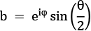
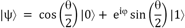
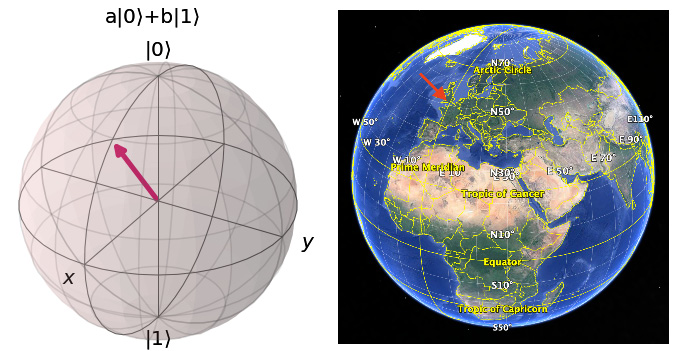
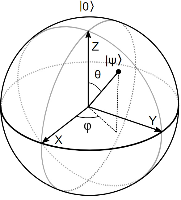
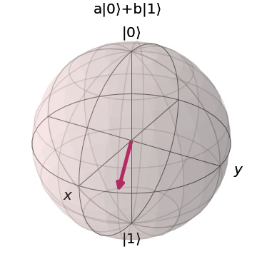
However, with a little mathematical trickery, it turns out that you can also describe a qubit using two angles—theta () and phi ()—and visualize the qubit on a Bloch sphere. You can think of the and angles much as the latitude and longitude of the earth. On the Bloch sphere, we can project any possible value that the qubit can take.

The equation for the transformation is as follows:

Here, we use the formula we saw before:

a and b are, respectively, as follows:

I'll leave the deeper details and math to you for further exploration:

Figure 2.2 – The Bloch sphere.

The poor classical bits cannot do much on a Bloch sphere as they can exist at the North and South poles only, representing the binary values 0 and 1. We will include them just for comparison.

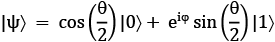
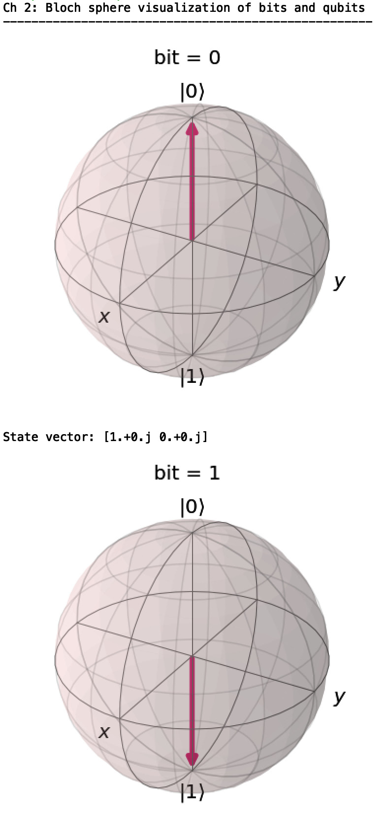
The reason 0 points up and 1 points down has peculiar and historical reasons. The qubit vector representation of is , or up, and is , or down, which is intuitively not what you expect. You would think that 1, or a more exciting qubit, would be a vector pointing upward, but this is not the case; it points down. So, I will do the same with the poor classical bits as well: 0 means up and 1 means down.

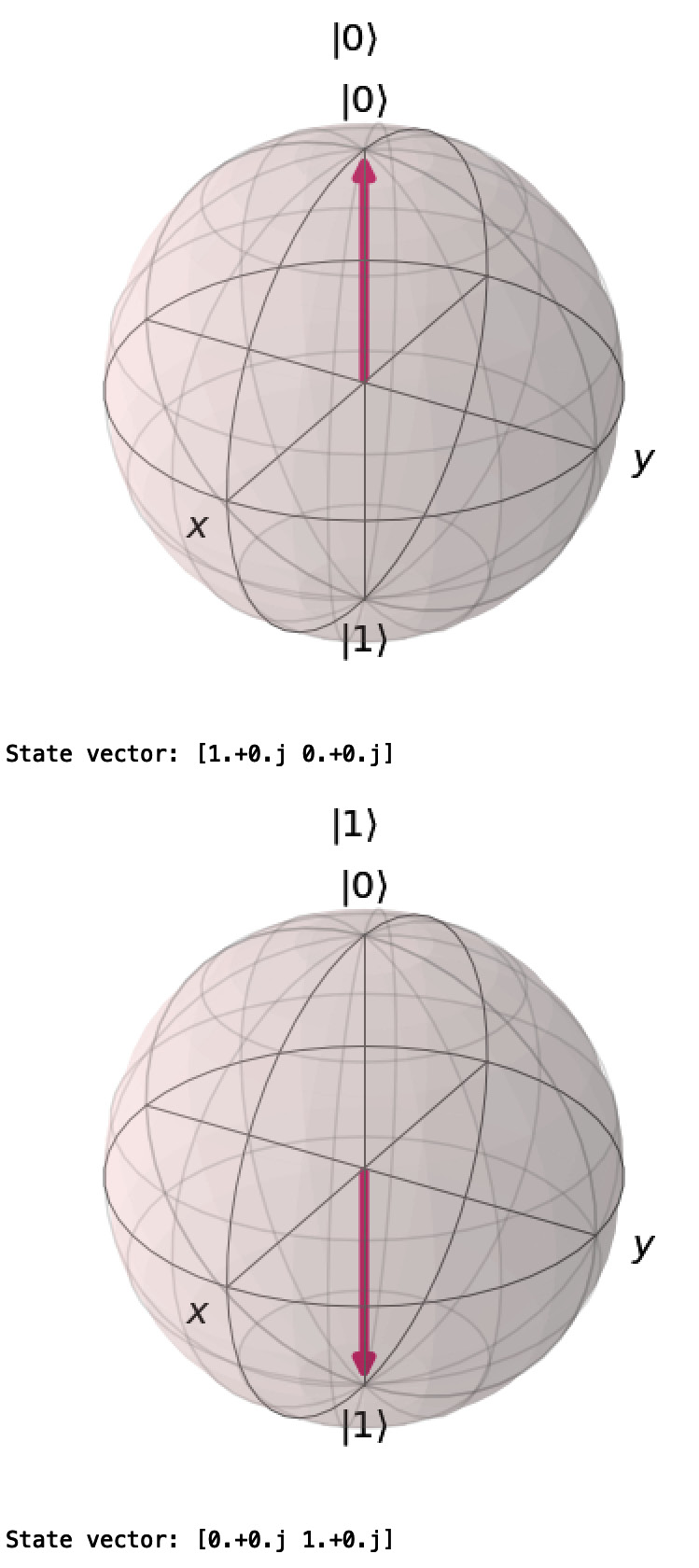
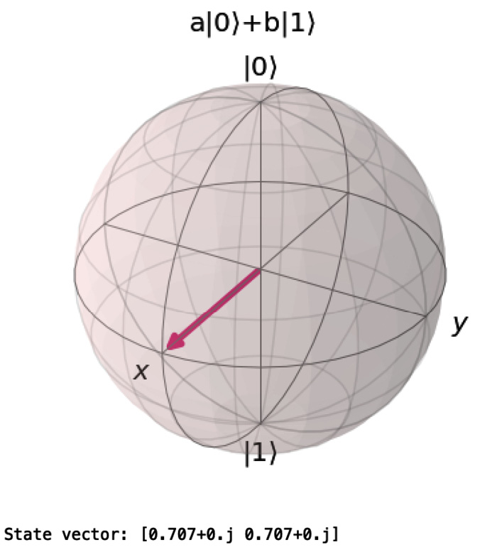
The latitude, the distance to the poles from a cut straight through the Bloch sphere, corresponds to the numerical values of a and b, with pointing straight up for (a=1, b=0), pointing straight down for 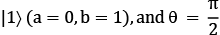points to the equator for the basic superposition where .

So, what we are adding to the equation here is the phase of the qubit. The angle cannot be directly measured and has no impact on the outcome of our initial quantum circuits. Later on in the book, in Chapter 9, Grover's Search Algorithm, we will see that you can use the phase angle to great advantage in certain algorithms. But we are getting ahead of ourselves.

Getting ready

The Python file for the following recipe can be downloaded from here: https://github.com/PacktPublishing/Quantum-Computing-in-Practice-with-Qiskit-and-IBM-Quantum-Experience/blob/master/Chapter02/ch2_r2_visualize_bits_qubits.py.

How to do it...

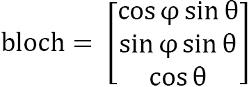
For this exercise, we will use the and angles as latitude and longitude coordinates on the Bloch sphere. We will code the 0, 1, , , and states with the corresponding angles. As we can set these angles to any latitude and longitude value we want, we can put the qubit state vector wherever we want on the Bloch sphere:

1. Import the classes and methods that we need, including numpy and plot_bloch_vector from Qiskit®. We also need to use cmath to do some calculations on imaginary numbers:

   import numpy as np
   import cmath 
   from math import pi, sin, cos
   from qiskit.visualization import plot_bloch_vector

2. Create the qubits:

   # Superposition with zero phase
   angles={"theta": pi/2, "phi":0}
   # Self defined qubit
   #angles["theta"]=float(input("Theta:\n"))
   #angles["phi"]=float(input("Phi:\n"))
   # Set up the bit and qubit vectors
   bits = {"bit = 0":{"theta": 0, "phi":0}, 
       "bit = 1":{"theta": pi, "phi":0}, 
       "|0\u27E9":{"theta": 0, "phi":0}, 
       "|1\u27E9":{"theta": pi, "phi":0}, 
       "a|0\u27E9+b|1\u27E9":angles}

   From the code sample, you can see that we are using the theta angle only for now, with theta = 0 meaning that we point straight up and theta meaning straight down for our basic bits and qubits: 0, 1, , and . Theta takes us halfway, to the equator, and we use that for the superposition qubit, .

3. Print the bits and qubits on the Bloch sphere.

   The Bloch sphere method takes a three-dimensional vector as input, but we have to build the vector first. We can use the following formula to calculate the X, Y, and Z parameters to use with plot_bloch_vector and display the bits and qubits as Bloch sphere representations:

   

   This is how it would look in our vector notation:

   

   And this is how we set this up in Python:

   bloch=[cos(bits[bit]["phi"])*sin(bits[bit]
       ["theta"]),sin(bits[bit]["phi"])*sin(bits[bit]
       ["theta"]),cos(bits[bit]["theta"])]

   We now cycle through the bits dictionary to display the Bloch sphere view of the bits and qubits, as well as the state vectors that correspond to them:

   

   The state vector is calculated using the equation we saw previously:

   

   What we see now is that a and b can actually turn into complex values, just as defined.

   Here's the code:

   for bit in bits:
        bloch=[cos(bits[bit]["phi"])*sin(bits[bit]
           ["theta"]),sin(bits[bit]["phi"])*sin(bits[bit]
           ["theta"]),cos(bits[bit]["theta"])]
       display(plot_bloch_vector(bloch, title=bit))
       # Build the state vector
       a = cos(bits[bit]["theta"]/2)
       b = cmath.exp(bits[bit]["phi"]*1j)*sin(bits[bit]
           ["theta"]/2)
       state_vector = [a * complex(1, 0), b * complex(1, 0)]
       print("State vector:", np.around(state_vector, 
           decimals = 3))

4. The sample code should give an output similar to the following examples.

   First, we show the classical bits, 0 and 1:

   

   Figure 2.3 – Bloch sphere visualization of classical bits

5. Then, we show the quantum bits, or qubits, and :
   

   Figure 2.4 – Bloch sphere visualization of qubits

6. Finally, we show a qubit in superposition, a mix of and :

Figure 2.5 – Bloch sphere visualization of a qubit in superposition

So, there is very little that is earth-shattering with the simple 0, 1, , and displays. They simply point up and down to the north and south pole of the Bloch sphere as appropriate. If we check what the value of the bit or qubit is by measuring it, we will get 0 or 1 with 100% certainty.

The qubit in superposition, calculated as , on the other hand, points to the equator. From the equator, it is an equally long distance to either pole, thus a 50/50 chance of getting a 0 or a 1.

In the code, we include the following few lines, which define the angles variable that sets and for the qubit:

# Superposition with zero phase
angles={"theta": pi/2, "phi":0}

There's more…

We mentioned earlier that we weren't going to touch on the phase () angle, at least not initially. But we can visualize what it does for our qubits. Remember that we can directly describe a and b using the angles and .

To test this out, you can uncomment the lines that define the angles in the sample code:

# Self-defined qubit
angles["theta"]=float(input("Theta:\n"))
angles["phi"]=float(input("Phi:\n"))

You can now define what your third qubit looks like by manipulating the and values. Let's test what we can do by running the script again and plugging in some angles.

For example, we can try the following:

You should see the final Bloch sphere look something like the following:

Figure 2.6 – The qubit state vector rotated by

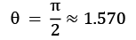
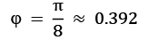
Note how the state vector is still on the equator with but now at angle to the x axis. You can also take a look at the state vector: [0.707+0.j 0.653+0.271j].

We have now stepped away from the Bloch sphere prime meridian and out into the complex plane, and added a phase angle, which is represented by an imaginary state vector component along the y axis:

Let's go on a trip

Go ahead and experiment with different and angles to get other a and b entries and see where you end up. No need to include 10+ decimals for these rough estimates, two or three decimals will do just fine. Try plotting your hometown on the Bloch sphere. Remember that the script wants the input in radians and that theta starts at the North Pole, not at the equator. For example, the coordinates for Greenwich Observatory in England are 51.4779° N, 0.0015° W, which translates into: , .

Here's Qiskit® and a globe displaying the same coordinates:

Figure 2.7 – Greenwich quantumly and on a globe

See also

Quantum Computation and Quantum Information, Isaac L. Chuang; Michael A. Nielsen, Cambridge University Press, 2010, Chapter 1.2, Quantum bits, and Chapter 4.2, Single qubit operations.