

Windows and Mac OS X users can run the R application to launch the R console. Linux and Mac OS X users can also run the R console straight from the Terminal by typing R.
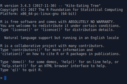
In either case, the R console itself will look something like the following screenshot:
R will respond to your commands right from the Terminal. Let's have a go. Run the following command in the R console:
> 2 + 2
[1] 4
The [1] phrase tells you that R returned one result, in this case, 4. The following command shows you how to print Hello world:
> print("Hello world!")
[1] "Hello world!"
The following command shows the multiples of pi:
> 1:10 * pi
[1]  3.141593  6.283185  9.424778 12.566371 15.707963 18.849556
[7] 21.991149 25.132741 28.274334 31.415927
This example illustrates vector-based programming in R. The 1:10 phrase generates the numbers 1:10 as a vector, and each is then multiplied by pi, which returns another vector, the elements each being pi times larger than the original. Operating on vectors is an important part of writing simple and efficient R code. As you can see, R again indexes the values it returns at the console, with the seventh value being 21.99.
One of the big strengths of using R is the graphics capability, which is excellent, even in a vanilla installation of R (these graphics are referred to as the base graphics because they ship with R). When adding packages such as ggplot2 and some of the JavaScript-based packages, R becomes a graphical tour de force, whether producing statistical, mathematical, or topographical figures, or indeed any other type of graphical output. To get a flavor of the power of the base graphics, simply type the following in the Console and see the types of plots that can be made using R:
> demo(graphics)
You can also type the following command:
> demo(persp)
There will be more on ggplot2 and base graphics later in the chapter.
Enjoy! There are many more examples of R graphics at r-graph-gallery.com.