

The intent of this chapter is not to make the reader an expert in statistical techniques. Rather, it is to familiarize the reader with the basic statistical techniques in use and demonstrate how Java can support statistical analysis. While there are quite a variety of data analysis techniques, in this chapter, we will focus on the more common tasks.
These techniques range from the relatively simple mean calculation to sophisticated regression analysis models. Statistical analysis can be a very complicated process and requires significant study to be conducted properly. We will start with an introduction to basic statistical analysis techniques, including calculating the mean, median, mode, and standard deviation of a dataset. There are numerous approaches used to calculate these values, which we will demonstrate using standard Java and third-party APIs. We will also briefly discuss sample size and hypothesis testing.
Regression analysis is an important technique for analyzing data. The technique creates a line that tries to match the dataset. The equation representing the line can be used to predict future behavior. There are several types of regression analysis. In this chapter, we will focus on simple linear regression and multiple regression. With simple linear regression, a single factor such as age is used to predict some behavior such as the likelihood of eating out. With multiple regression, multiple factors such as age, income level, and marital status may be used to predict how often a person eats out.
Predictive analytics, or analysis, is concerned with predicting future events. Many of the techniques used in this book are concerned with making predictions. Specifically, the regression analysis part of this chapter predicts future behavior.
Before we see how Java supports regression analysis, we need to discuss basic statistical techniques. We begin with mean, mode, and median.
In this chapter, we will cover the following topics:
- Working with mean, mode, and median
- Standard deviation and sample size determination
- Hypothesis testing
- Regression analysis
The mean, median, and mode are basic ways to describe characteristics or summarize information from a dataset. When a new, large dataset is first encountered, it can be helpful to know basic information about it to direct further analysis. These values are often used in later analysis to generate more complex measurements and conclusions. This can occur when we use the mean of a dataset to calculate the standard deviation, which we will demonstrate in the Standard deviation section of this chapter.
The term mean, also called the average, is computed by adding values in a list and then dividing the sum by the number of values. This technique is useful for determining the general trend for a set of numbers. It can also be used to fill in missing data elements. We are going to examine several ways to calculate the mean for a given set of data using standard Java libraries as well as third-party APIs.
In our first example, we will demonstrate a basic way to calculate mean using standard Java capabilities. We will use an array of double values called testData:
double[] testData = {12.5, 18.7, 11.2, 19.0, 22.1, 14.3, 16.9, 12.5,
17.8, 16.9};
We create a double variable to hold the sum of all of the values and a double variable to hold the mean. A loop is used to iterate through the data and add values together. Next, the sum is divided by the length of our array (the total number of elements) to calculate the mean:
double total = 0;
for (double element : testData) {
total += element;
}
double mean = total / testData.length;
out.println("The mean is " + mean);
Our output is as follows:
The mean is 16.19
Java 8 provided additional capabilities with the introduction of optional classes. We are going to use the OptionalDouble class in conjunction with the Arrays class's stream method in this example. We will use the same array of doubles we used in the previous example to create an OptionalDouble object. If any of the numbers in the array, or the sum of the numbers in the array, is not a real number, the value of the OptionalDouble object will also not be a real number:
OptionalDouble mean = Arrays.stream(testData).average();
We use the isPresent method to determine whether we calculated a valid number for our mean. If we do not get a good result, the isPresent method will return false and we can handle any exceptions:
if (mean.isPresent()) {
out.println("The mean is " + mean.getAsDouble());
} else {
out.println("The stream was empty");
}
Our output is the following:
The mean is 16.19
Another, more succinct, technique using the OptionalDouble class involves lambda expressions and the ifPresent method. This method executes its argument if mean is a valid OptionalDouble object:
OptionalDouble mean = Arrays.stream(testData).average();
mean.ifPresent(x-> out.println("The mean is " + x));
Our output is as follows:
The mean is 16.19
Finally, we can use the orElse method to either print the mean or an alternate value if mean is not a valid OptionalDouble object:
OptionalDouble mean = Arrays.stream(testData).average();
out.println("The mean is " + mean.orElse(0));
Our output is the same:
The mean is 16.19
For our next two mean examples, we will use third-party libraries and continue using the array of doubles, testData.
In this example, we will use Google Guava libraries, introduced in Chapter 3, Data Cleaning. The Stats class provides functionalities for handling numeric data, including finding mean and standard deviation, which we will demonstrate later. To calculate the mean, we first create a Stats object using our testData array and then execute the mean method:
Stats testStat = Stats.of(testData);
double mean = testStat.mean();
out.println("The mean is " + mean);
Notice the difference between the default format of the output in this example.
In our final mean examples, we use Apache Commons libraries, also introduced in Chapter 3, Data Cleaning. We first create a Mean object and then execute the evaluate method using our testData. This method returns a double
, representing the mean of the values in the array:
Mean mean = new Mean();
double average = mean.evaluate(testData);
out.println("The mean is " + average);
Our output is the following:
The mean is 16.19
Apache Commons also provides a helpful DescriptiveStatistics class. We will use this later to demonstrate median and standard deviation, but first we will begin by calculating the mean. Using the SynchronizedDescriptiveStatistics class is advantageous as it is synchronized and therefore thread safe.
We start by creating our DescriptiveStatistics object, statTest. We then loop through our double array and add each item to statTest. We can then invoke the getMean method to calculate the mean:
DescriptiveStatistics statTest =
new SynchronizedDescriptiveStatistics();
for(double num : testData){
statTest.addValue(num);
}
out.println("The mean is " + statTest.getMean());
Our output is as follows:
The mean is 16.19
Next, we will cover the related topic: median.
The mean can be misleading if the dataset contains a large number of outlying values or is otherwise skewed. When this happens, the mode and median can be useful. The term median is the value in the middle of a range of values. For an odd number of values, this is easy to compute. For an even number of values, the median is calculated as the average of the middle two values.
In our first example, we will use a basic Java approach to calculate the median. For these examples, we have modified our testData array slightly:
double[] testData = {12.5, 18.3, 11.2, 19.0, 22.1, 14.3, 16.2, 12.5,
17.8, 16.5};
First, we use the Arrays class to sort our data because finding the median is simplified when the data is in numeric order:
Arrays.sort(testData);
We then handle three possibilities:
- Our list is empty
- Our list has an even number of values
- Our list has an odd number of values
The following code could be shortened, but we have been explicit to help clarify the process. If our list has an even number of values, we divide the length of the list by 2. The first variable, mid1, will hold the first of two middle values. The second variable, mid2, will hold the second middle value. The average of these two numbers is our median value. The process for finding the median index of a list with an odd number of values is simpler and requires only that we divide the length by 2 and add 1:
if(testData.length==0){ // Empty list
out.println("No median. Length is 0");
}else if(testData.length%2==0){ // Even number of elements
double mid1 = testData[(testData.length/2)-1];
double mid2 = testData[testData.length/2];
double med = (mid1 + mid2)/2;
out.println("The median is " + med);
}else{ // Odd number of elements
double mid = testData[(testData.length/2)+1];
out.println("The median is " + mid);
}
Using the preceding array, which contains an even number of values, our output is:
The median is 16.35
To test our code for an odd number of elements, we will add the double 12.5 to the end of the array. Our new output is as follows:
The median is 16.5
We can also calculate the median using the Apache Commons DescriptiveStatistics class demonstrated in the Calculating the mean section. We will continue using the testData array with the following values:
double[] testData = {12.5, 18.3, 11.2, 19.0, 22.1, 14.3, 16.2, 12.5,
17.8, 16.5, 12.5};
Our code is very similar to what we used to calculate the mean. We simply create our DescriptiveStatistics object and call the getPercentile method, which returns an estimate of the value stored at the percentile specified in its argument. To find the median, we use the value of 50:
DescriptiveStatistics statTest =
new SynchronizedDescriptiveStatistics();
for(double num : testData){
statTest.addValue(num);
}
out.println("The median is " + statTest.getPercentile(50));
Our output is as follows:
The median is 16.2
The term mode is used for the most frequently occurring value in a dataset. This can be thought of as the most popular result, or the highest bar in a histogram. It can be a useful piece of information when conducting statistical analysis but it can be more complicated to calculate than it first appears. To begin, we will demonstrate a simple Java technique using the following testData array:
double[] testData = {12.5, 18.3, 11.2, 19.0, 22.1, 14.3, 16.2, 12.5,
17.8, 16.5, 12.5};
We start off by initializing variables to hold the mode, the number of times the mode appears in the list, and a tempCnt variable. The mode and modeCount variables are used to hold the mode value and the number of times this value occurs in the list respectively. The variable tempCnt is used to count the number of times an element occurs in the list:
int modeCount = 0; double mode = 0; int tempCnt = 0;
We then use nested for loops to compare each value of the array to the other values within the array. When we find matching values, we increment our tempCnt. After comparing each value, we test to see whether tempCnt is greater than modeCount, and if so, we change our modeCount and mode to reflect the new values:
for (double testValue : testData){
tempCnt = 0;
for (double value : testData){
if (testValue == value){
tempCnt++;
}
}
if (tempCnt > modeCount){
modeCount = tempCnt;
mode = testValue;
}
}
out.println("Mode" + mode + " appears " + modeCount + " times.");
Using this example, our output is as follows:
The mode is 12.5 and appears 3 times.
While our preceding example seems straightforward, it poses potential problems. Modify the testData array as shown here, where the last entry is changed to 11.2:
double[] testData = {12.5, 18.3, 11.2, 19.0, 22.1, 14.3, 16.2, 12.5,
17.8, 16.5, 11.2};
When we execute our code this time, our output is as follows:
The mode is 12.5 and appears 2 times.
The problem is that our testData array now contains two values that appear two times each, 12.5 and 11.2. This is known as a multimodal set of data. We can address this through basic Java code and through third-party libraries, as we will show in a moment.
However, first we will show two approaches using simple Java. The first approach will use two ArrayList instances and the second will use an ArrayList and a HashMap instance.
In the first approach, we modify the code used in the last example to use an ArrayList class. We will create two ArrayLists, one to hold the unique numbers within the dataset and one to hold the count of each number. We also need a tempMode variable, which we use next:
ArrayList<Integer> modeCount = new ArrayList<Integer>(); ArrayList<Double> mode = new ArrayList<Double>(); int tempMode = 0;
Next, we will loop through the array and test for each value in our mode list. If the value is not found in the list, we add it to mode and set the same position in modeCount to 1. If the value is found, we increment the same position in modeCount by 1:
for (double testValue : testData){
int loc = mode.indexOf(testValue);
if(loc == -1){
mode.add(testValue);
modeCount.add(1);
}else{
modeCount.set(loc, modeCount.get(loc)+1);
}
}
Next, we loop through our modeCount list to find the largest value. This represents the mode, or the frequency of the most common value in the dataset. This allows us to select multiple modes:
for(int cnt = 0; cnt < modeCount.size(); cnt++){
if (tempMode < modeCount.get(cnt)){
tempMode = modeCount.get(cnt);
}
}
Finally, we loop through our modeCount array again and print out any elements in mode that correspond to elements in modeCount containing the largest value, or mode:
for(int cnt = 0; cnt < modeCount.size(); cnt++){
if (tempMode == modeCount.get(cnt)){
out.println(mode.get(cnt) + " is a mode and appears " +
modeCount.get(cnt) + " times.");
}
}
When our code is executed, our output reflects our multimodal dataset:
12.5 is a mode and appears 2 times. 11.2 is a mode and appears 2 times.
The second approach uses HashMap. First, we create ArrayList to hold possible modes, as in the previous example. We also create our HashMap and a variable to hold the mode:
ArrayList<Double> modes = new ArrayList<Double>(); HashMap<Double, Integer> modeMap = new HashMap<Double, Integer>(); int maxMode = 0;
Next, we loop through our testData array and count the number of occurrences of each value in the array. We then add the count of each value and the value itself to the HashMap. If the count for the value is larger than our maxMode variable, we set maxMode to our new largest number:
for (double value : testData) {
int modeCnt = 0;
if (modeMap.containsKey(value)) {
modeCnt = modeMap.get(value) + 1;
} else {
modeCnt = 1;
}
modeMap.put(value, modeCnt);
if (modeCnt > maxMode) {
maxMode = modeCnt;
}
}
Finally, we loop through our HashMap and retrieve our modes, or all values with a count equal to our maxMode:
for (Map.Entry<Double, Integer> multiModes : modeMap.entrySet()) {
if (multiModes.getValue() == maxMode) {
modes.add(multiModes.getKey());
}
}
for(double mode : modes){
out.println(mode + " is a mode and appears " + maxMode + " times.");
}
When we execute our code, we get the same output as in the previous example:
12.5 is a mode and appears 2 times. 11.2 is a mode and appears 2 times.
Another option uses the Apache Commons StatUtils class. This class contains several methods for statistical analysis, including multiple methods for the mean, but we will only examine the mode here. The method is named mode and takes an array of doubles as its parameter. It returns an array of doubles containing all modes of the dataset:
double[] modes = StatUtils.mode(testData);
for(double mode : modes){
out.println(mode + " is a mode.");
}
One disadvantage is that we are not able to count the number of times our mode appears within this method. We simply know what the mode is, not how many times it appears. When we execute our code, we get a similar output to our previous example:
12.5 is a mode. 11.2 is a mode.
Standard deviation is a measurement of how values are spread around the mean. A high deviation means that there is a wide spread, whereas a low deviation means that the values are more tightly grouped around the mean. This measurement can be misleading if there is not a single focus point or there are numerous outliers.
We begin by showing a simple example using basic Java techniques. We are using our testData array from previous examples, duplicated here:
double[] testData = {12.5, 18.3, 11.2, 19.0, 22.1, 14.3, 16.2, 12.5,
17.8, 16.5, 11.2};
Before we can calculate the standard deviation, we need to find the average. We could use any of our techniques listed in the Calculating the mean section, but we will add up our values and divide by the length of testData for simplicity's sake:
int sum = 0;
for(double value : testData){
sum += value;
}
double mean = sum/testData.length;
Next, we create a variable, sdSum, to help us calculate the standard deviation. As we loop through our array, we subtract the mean from each data value, square that value, and add it to sdSum. Finally, we divide sdSum by the length of the array and square that result:
int sdSum = 0;
for (double value : testData){
sdSum += Math.pow((value - mean), 2);
}
out.println("The standard deviation is " +
Math.sqrt( sdSum / ( testData.length ) ));
Our output is our standard deviation:
The standard deviation is 3.3166247903554
Our next technique uses Google Guava's Stats class to calculate the standard deviation. We start by creating a Stats object with our testData. We then call the populationStandardDeviation method:
Stats testStats = Stats.of(testData);
double sd = testStats.populationStandardDeviation();
out.println("The standard deviation is " + sd);
The output is as follows:
The standard deviation is 3.3943803826056653
This example calculates the standard deviation of an entire population. Sometimes it is preferable to calculate the standard deviation of a sample subset of a population, to correct possible bias. To accomplish this, we use essentially the same code as before but replace the populationStandardDeviation method with sampleStandardDeviation:
Stats testStats = Stats.of(testData);
double sd = testStats.sampleStandardDeviation();
out.println("The standard deviation is " + sd);
In this case, our output is:
The sample standard deviation is 3.560056179332006
Our next example uses the Apache Commons DescriptiveStatistics class, which we used to calculate the mean and median in previous examples. Remember, this technique has the advantage of being thread safe and synchronized. After we create a SynchronizedDescriptiveStatistics object, we add each value from the array. We then call the getStandardDeviation method.
DescriptiveStatistics statTest =
new SynchronizedDescriptiveStatistics();
for(double num : testData){
statTest.addValue(num);
}
out.println("The standard deviation is " +
statTest.getStandardDeviation());
Notice the output matches our output from our previous example. The getStandardDeviation method by default returns the standard deviation adjusted for a sample:
The standard deviation is 3.5600561793320065
We can, however, continue using Apache Commons to calculate the standard deviation in either form. The StandardDeviation class allows you to calculate the population standard deviation or subset standard deviation. To demonstrate the differences, replace the previous code example with the following:
StandardDeviation sdSubset = new StandardDeviation(false);
out.println("The population standard deviation is " +
sdSubset.evaluate(testData));
StandardDeviation sdPopulation = new StandardDeviation(true);
out.println("The sample standard deviation is " +
sdPopulation.evaluate(testData));
On the first line, we created a new StandardDeviation object and set our constructor's parameter to false, which will produce the standard deviation of a population. The second section uses a value of true, which produces the standard deviation of a sample. In our example, we used the same test dataset. This means we were first treating it as though it were a subset of a population of data. In our second example we assumed that our dataset was the entire population of data. In reality, you would might not use the same set of data with each of those methods. The output is as follows:
The population standard deviation is 3.3943803826056653 The sample standard deviation is 3.560056179332006
The preferred option will depend upon your sample and particular analyzation needs.
Sample size determination involves identifying the quantity of data required to conduct accurate statistical analysis. When working with large datasets it is not always necessary to use the entire set. We use sample size determination to ensure we choose a sample small enough to manipulate and analyze easily, but large enough to represent our population of data accurately.
It is not uncommon to use a subset of data to train a model and another subset is used to test the model. This can be helpful for verifying accuracy and reliability of data. Some common consequences for a poorly determined sample size include false-positive results, false-negative results, identifying statistical significance where none exists, or suggesting a lack of significance where it is actually present. Many tools exist online for determining appropriate sample sizes, each with varying levels of complexity. One simple example is available at https://www.surveymonkey.com/mp/sample-size-calculator/.
Hypothesis testing is used to test whether certain assumptions, or premises, about a dataset could not happen by chance. If this is the case, then the results of the test are considered to be statistically significant.
Performing hypothesis testing is not a simple task. There are many different pitfalls to avoid such as the placebo effect or the observer effect. In the former, a participant will attain a result that they think is expected. In the observer effect, also called the Hawthorne effect, the results are skewed because the participants know they are being watched. Due to the complex nature of human behavior analysis, some types of statistical analysis are particularly subject to skewing or corruption.
The specific methods for performing hypothesis testing are outside the scope of this book and require a solid background in statistical processes and best practices. Apache Commons provides a package, org.apache.commons.math3.stat.inference, with tools for performing hypothesis testing. This includes tools to perform a student's T-test, chi square, and calculating p values.
Regression analysis is useful for determining trends in data. It indicates the relationship between dependent and independent variables. The independent variables determine the value of a dependent variable. Each independent variable can have either a strong or a weak effect on the value of the dependent variable. Linear regression uses a line in a scatterplot to show the trend. Non-linear regression uses some sort of curve to depict the relationships.
For example, there is a relationship between blood pressure and various factors such as age, salt intake, and Body Mass Index (BMI). The blood pressure can be treated as the dependent variable and the other factors as independent variables. Given a dataset containing these factors for a group of individuals we can perform regression analysis to see trends.
There are several types of regression analysis supported by Java. We will be examining simple linear regression and multiple linear regression. Both approaches take a dataset and derive a linear equation that best fits the data. Simple linear regression uses a single dependent and a single independent variable. Multiple linear regression uses multiple dependent variables.
There are several APIs that support simple linear regression including:
- Apache Commons - http://commons.apache.org/proper/commons-math/javadocs/api-3.6.1/index.html
- Weka - http://weka.sourceforge.net/doc.dev/weka/core/matrix/LinearRegression.html
- JFree - http://www.jfree.org/jfreechart/api/javadoc/org/jfree/data/statistics/Regression.html
- Michael Thomas Flanagan's Java Scientific Library - http://www.ee.ucl.ac.uk/~mflanaga/java/Regression.html
Nonlinear Java support can be found at:
- odinsbane/least-squares-in-java - https://github.com/odinsbane/least-squares-in-java
- NonLinearLeastSquares (Parallel Java Library Documentation) - https://www.cs.rit.edu/~ark/pj/doc/edu/rit/numeric/NonLinearLeastSquares.html
There are several statistics that evaluate the effectiveness of an analysis. We will focus on basic statistics.
Residuals are the difference between the actual data values and the predicted values. The Residual Sum of Squares (RSS) is the sum of the squares of residuals. Essentially it measures the discrepancy between the data and a regression model. A small RSS indicates the model closely matches the data. RSS is also known as the Sum of Squared Residuals (SSR) or the Sum of Squared Errors (SSE) of prediction.
The Mean Square Error (MSE) is the sum of squared residuals divided by the degrees of freedom. The number of degrees of freedom is the number of independent observations (N) minus the number of estimates of population parameters. For simple linear regression this N - 2 because there are two parameters. For multiple linear regression it depends on the number of independent variables used.
A small MSE also indicates that the model fits the dataset well. You will see both of these statistics used when discussing linear regression models.
The correlation coefficient measures the association between two variables of a regression model. The correlation coefficient ranges from -1 to +1. A value of +1 means that two variables are perfectly related. When one increases, so does the other. A correlation coefficient of -1 means that two variables are negatively related. When one increases, the other decreases. A value of 0 means there is no correlation between the variables. The coefficient is frequently designated as R. It will often be squared, thus ignoring the sign of the relation. The Pearson's product moment correlation coefficient is normally used.
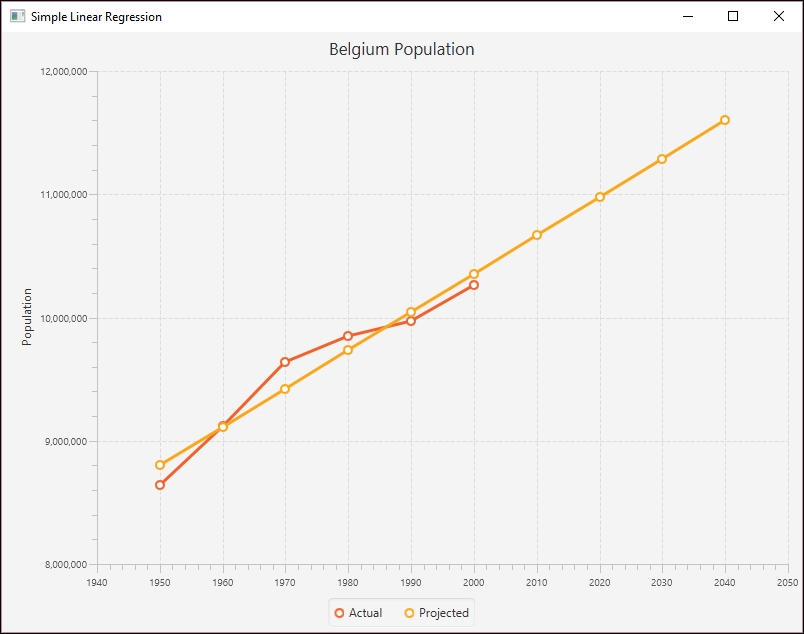
Simple linear regression uses a least squares approach where a line is computed that minimizes the sum of squared of the distances between the points and the line. Sometimes the line is calculated without using the Y intercept term. The regression line is an estimate. We can use the line's equation to predict other data points. This is useful when we want to predict future events based on past performance.
In the following example we use the Apache Commons SimpleRegression class with the Belgium population dataset used in Chapter 4, Data Visualization. The data is duplicated here for your convenience:
|
Decade |
Population |
|
|
|
|
|
|
|
|
|
|
|
|
|
|
|
|
|
|
While the application that we will demonstrate is a JavaFX application, we will focus on the linear regression aspects of the application. We used a JavaFX program to generate a chart to show the regression results.
The body of the start method follows. The input data is stored in a two-dimension array as shown here:
double[][] input = {{1950, 8639369}, {1960, 9118700},
{1970, 9637800}, {1980, 9846800}, {1990, 9969310},
{2000, 10263618}};
An instance of the SimpleRegression class is created and the data is added using the addData method:
SimpleRegression regression = new SimpleRegression(); regression.addData(input);
We will use the model to predict behavior for several years as declared in the array that follows:
double[] predictionYears = {1950, 1960, 1970, 1980, 1990, 2000,
2010, 2020, 2030, 2040};
We will also format our output using the following NumberFormat instances. One is used for the year where the setGroupingUsed method with a parameter of false suppresses commas.
NumberFormat yearFormat = NumberFormat.getNumberInstance(); yearFormat.setMaximumFractionDigits(0); yearFormat.setGroupingUsed(false); NumberFormat populationFormat = NumberFormat.getNumberInstance(); populationFormat.setMaximumFractionDigits(0);
The SimpleRegression class possesses a predict method that is passed a value, a year in this case, and returns the estimated population. We use this method in a loop and call the method for each year:
for (int i = 0; i < predictionYears.length; i++) {
out.println(nf.format(predictionYears[i]) + "-"
+ nf.format(regression.predict(predictionYears[i])));
}
When the program is executed, we get the following output:
1950-8,801,975 1960-9,112,892 1970-9,423,808 1980-9,734,724 1990-10,045,641 2000-10,356,557 2010-10,667,474 2020-10,978,390 2030-11,289,307 2040-11,600,223
To see the results graphically, we generated the following index chart. The line matches the actual population values fairly well and shows the projected populations in the future.
Simple Linear Regression
The SimpleRegession class supports a number of methods that provide additional information about the regression. These methods are summarized next:
|
Method |
Meaning |
|
|
Returns Pearson's product moment correlation coefficient |
|
|
Returns the coefficient of determination (R-square) |
|
|
Returns the MSE |
|
|
The slope of the line |
|
|
The intercept |
We used the helper method, displayAttribute, to display various attribute values as shown here:
displayAttribute(String attribute, double value) {
NumberFormat numberFormat = NumberFormat.getNumberInstance();
numberFormat.setMaximumFractionDigits(2);
out.println(attribute + ": " + numberFormat.format(value));
}
We called the previous methods for our model as shown next:
displayAttribute("Slope",regression.getSlope());
displayAttribute("Intercept", regression.getIntercept());
displayAttribute("MeanSquareError",
regression.getMeanSquareError());
displayAttribute("R", + regression.getR());
displayAttribute("RSquare", regression.getRSquare());
The output follows:
Slope: 31,091.64 Intercept: -51,826,728.48 MeanSquareError: 24,823,028,973.4 R: 0.97 RSquare: 0.94
As you can see, the model fits the data nicely.
Our intent is not to provide a detailed explanation of multiple linear regression as that would be beyond the scope of this section. A more through treatment can be found athttp://www.biddle.com/documents/bcg_comp_chapter4.pdf. Instead, we will explain the basics of the approach and show how we can use Java to perform multiple regression.
Multiple regression works with data where multiple independent variables exist. This happens quite often. Consider that the fuel efficiency of a car can be dependent on the octane level of the gas being used, the size of the engine, the average cruising speed, and the ambient temperature. All of these factors can influence the fuel efficiency, some to a larger degree than others.
The independent variable is normally represented as Y where there are multiple dependent variables represented using different Xs. A simplified equation for a regression using three dependent variables follows where each variable has a coefficient. The first term is the intercept. These coefficients are not intended to represent real values but are only used for illustrative purposes.
Y = 11 + 0.75 X1 + 0.25 X2 − 2 X3
The intercept and coefficients are generated using a multiple regression model based on sample data. Once we have these values, we can create an equation to predict other values.
We will use the Apache Commons OLSMultipleLinearRegression class to perform multiple regression using cigarette data. The data has been adapted from http://www.amstat.org/publications/jse/v2n1/datasets.mcintyre.html. The data consists of 25 entries for different brands of cigarettes with the following information:
- Brand name
- Tar content (mg)
- Nicotine content (mg)
- Weight (g)
- Carbon monoxide content (mg)
The data has been stored in a file called data.csv as shown in the following partial listing of its contents where the columns values match the order of the previous list:
Alpine,14.1,.86,.9853,13.6 Benson&Hedges,16.0,1.06,1.0938,16.6 BullDurham,29.8,2.03,1.1650,23.5 CamelLights,8.0,.67,.9280,10.2 ...
The following is a scatter plot chart showing the relationship of the data:
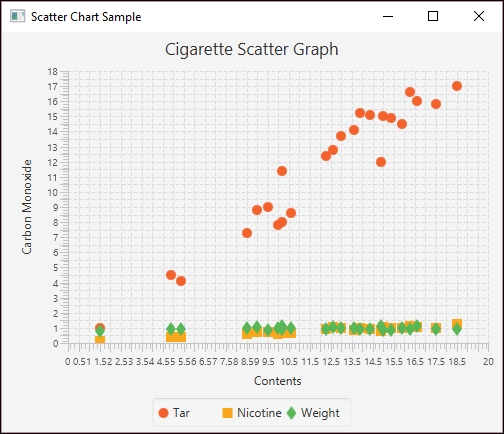
Multiple Regression Scatter plot
We will use a JavaFX program to create the scatter plot and to perform the analysis. We start with the
MainApp class as shown next. In this example we will focus on the multiple regression code and we do not include the JavaFX code used to create the scatter plot. The complete program can be downloaded from http://www.packtpub.com/support.
The data is held in a one-dimensional array and a NumberFormat instance will be used to format the values. The array size reflects the 25 entries and the 4 values per entry. We will not be using the brand name in this example.
public class MainApp extends Application {
private final double[] data = new double[100];
private final NumberFormat numberFormat =
NumberFormat.getNumberInstance();
...
public static void main(String[] args) {
launch(args);
}
}The data is read into the array using a CSVReader instance as shown next:
int i = 0; try (CSVReader dataReader = new CSVReader( new FileReader("data.csv"), ',')) { String[] nextLine; while ((nextLine = dataReader.readNext()) != null) { String brandName = nextLine[0]; double tarContent = Double.parseDouble(nextLine[1]); double nicotineContent = Double.parseDouble(nextLine[2]); double weight = Double.parseDouble(nextLine[3]); double carbonMonoxideContent = Double.parseDouble(nextLine[4]); data[i++] = carbonMonoxideContent; data[i++] = tarContent; data[i++] = nicotineContent; data[i++] = weight; ... } }
Apache Commons possesses two classes that perform multiple regression:
-
OLSMultipleLinearRegression- Ordinary Least Square (OLS) regression GLSMultipleLinearRegression- Generalized Least Squared (GLS) regression
When the latter technique is used, the correlation within elements of the model impacts the results addversely. We will use the OLSMultipleLinearRegression class and start with its instantiation:
OLSMultipleLinearRegression ols = new OLSMultipleLinearRegression();
We will use the newSampleData method to initialize the model. This method needs the number of observations in the dataset and the number of independent variables. It may throw an IllegalArgumentException exception which needs to be handled.
int numberOfObservations = 25; int numberOfIndependentVariables = 3; try { ols.newSampleData(data, numberOfObservations, numberOfIndependentVariables); } catch (IllegalArgumentException e) { // Handle exceptions }
Next, we set the number of digits that will follow the decimal point to two and invoke the estimateRegressionParameters method. This returns an array of values for our equation, which are then displayed:
numberFormat.setMaximumFractionDigits(2); double[] parameters = ols.estimateRegressionParameters(); for (int i = 0; i < parameters.length; i++) { out.println("Parameter " + i +": " + numberFormat.format(parameters[i])); }
When executed we will get the following output which gives us the parameters needed for our regression equation:
Parameter 0: 3.2 Parameter 1: 0.96 Parameter 2: -2.63 Parameter 3: -0.13
To predict a new dependent value based on a set of independent variables, the getY method is declared, as shown next. The parameters parameter contains the generated equation coefficients. The arguments parameter contains the value for the dependent variables. These are used to calculate the new dependent value which is returned:
public double getY(double[] parameters, double[] arguments) { double result = 0; for(int i=0; i<parameters.length; i++) { result += parameters[i] * arguments[i]; } return result; }
We can test this method by creating a series of independent values. Here we used the same values as used for the SalemUltra entry in the data file:
double arguments1[] = {1, 4.5, 0.42, 0.9106}; out.println("X: " + 4.9 + " y: " + numberFormat.format(getY(parameters,arguments1)));
This will give us the following values:
X: 4.9 y: 6.31
The return value of 6.31 is different from the actual value of 4.9. However, using the values for VirginiaSlims:
double arguments2[] = {1, 15.2, 1.02, 0.9496}; out.println("X: " + 13.9 + " y: " + numberFormat.format(getY(parameters,arguments2)));
We get the following result:
X: 13.9 y: 15.03
This is close to the actual value of 13.9. Next, we use a different set of values than found in the dataset:
double arguments3[] = {1, 12.2, 1.65, 0.86}; out.println("X: " + 9.9 + " y: " + numberFormat.format(getY(parameters,arguments3)));
The result follows:
X: 9.9 y: 10.49
The values differ but are still close. The following figure shows the predicted data in relation to the original data:
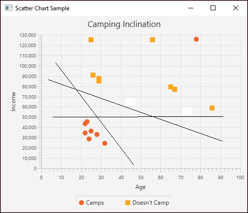
Multiple regression projected
The OLSMultipleLinearRegression class also possesses several methods to evaluate how well the models fits the data. However, due to the complex nature of multiple regression, we have not discussed them here.
Using simple linear regression
Simple linear regression uses a least squares approach where a line is computed that minimizes the sum of squared of the distances between the points and the line. Sometimes the line is calculated without using the Y intercept term. The regression line is an estimate. We can use the line's equation to predict other data points. This is useful when we want to predict future events based on past performance.
In the following example we use the Apache Commons SimpleRegression class with the Belgium population dataset used in Chapter 4, Data Visualization. The data is duplicated here for your convenience:
|
Decade |
Population |
|
|
|
|
|
|
|
|
|
|
|
|
|
|
|
|
|
|
While the application that we will demonstrate is a JavaFX application, we will focus on the linear regression aspects of the application. We used a JavaFX program to generate a chart to show the regression results.
The body of the start method follows. The input data is stored in a two-dimension array as shown here:
double[][] input = {{1950, 8639369}, {1960, 9118700},
{1970, 9637800}, {1980, 9846800}, {1990, 9969310},
{2000, 10263618}};
An instance of the SimpleRegression class is created and the data is added using the addData method:
SimpleRegression regression = new SimpleRegression(); regression.addData(input);
We will use the model to predict behavior for several years as declared in the array that follows:
double[] predictionYears = {1950, 1960, 1970, 1980, 1990, 2000,
2010, 2020, 2030, 2040};
We will also format our output using the following NumberFormat instances. One is used for the year where the setGroupingUsed method with a parameter of false suppresses commas.
NumberFormat yearFormat = NumberFormat.getNumberInstance(); yearFormat.setMaximumFractionDigits(0); yearFormat.setGroupingUsed(false); NumberFormat populationFormat = NumberFormat.getNumberInstance(); populationFormat.setMaximumFractionDigits(0);
The SimpleRegression class possesses a predict method that is passed a value, a year in this case, and returns the estimated population. We use this method in a loop and call the method for each year:
for (int i = 0; i < predictionYears.length; i++) {
out.println(nf.format(predictionYears[i]) + "-"
+ nf.format(regression.predict(predictionYears[i])));
}
When the program is executed, we get the following output:
1950-8,801,975 1960-9,112,892 1970-9,423,808 1980-9,734,724 1990-10,045,641 2000-10,356,557 2010-10,667,474 2020-10,978,390 2030-11,289,307 2040-11,600,223
To see the results graphically, we generated the following index chart. The line matches the actual population values fairly well and shows the projected populations in the future.
Simple Linear Regression
The SimpleRegession class supports a number of methods that provide additional information about the regression. These methods are summarized next:
|
Method |
Meaning |
|
|
Returns Pearson's product moment correlation coefficient |
|
|
Returns the coefficient of determination (R-square) |
|
|
Returns the MSE |
|
|
The slope of the line |
|
|
The intercept |
We used the helper method, displayAttribute, to display various attribute values as shown here:
displayAttribute(String attribute, double value) {
NumberFormat numberFormat = NumberFormat.getNumberInstance();
numberFormat.setMaximumFractionDigits(2);
out.println(attribute + ": " + numberFormat.format(value));
}
We called the previous methods for our model as shown next:
displayAttribute("Slope",regression.getSlope());
displayAttribute("Intercept", regression.getIntercept());
displayAttribute("MeanSquareError",
regression.getMeanSquareError());
displayAttribute("R", + regression.getR());
displayAttribute("RSquare", regression.getRSquare());
The output follows:
Slope: 31,091.64 Intercept: -51,826,728.48 MeanSquareError: 24,823,028,973.4 R: 0.97 RSquare: 0.94
As you can see, the model fits the data nicely.
Our intent is not to provide a detailed explanation of multiple linear regression as that would be beyond the scope of this section. A more through treatment can be found athttp://www.biddle.com/documents/bcg_comp_chapter4.pdf. Instead, we will explain the basics of the approach and show how we can use Java to perform multiple regression.
Multiple regression works with data where multiple independent variables exist. This happens quite often. Consider that the fuel efficiency of a car can be dependent on the octane level of the gas being used, the size of the engine, the average cruising speed, and the ambient temperature. All of these factors can influence the fuel efficiency, some to a larger degree than others.
The independent variable is normally represented as Y where there are multiple dependent variables represented using different Xs. A simplified equation for a regression using three dependent variables follows where each variable has a coefficient. The first term is the intercept. These coefficients are not intended to represent real values but are only used for illustrative purposes.
Y = 11 + 0.75 X1 + 0.25 X2 − 2 X3
The intercept and coefficients are generated using a multiple regression model based on sample data. Once we have these values, we can create an equation to predict other values.
We will use the Apache Commons OLSMultipleLinearRegression class to perform multiple regression using cigarette data. The data has been adapted from http://www.amstat.org/publications/jse/v2n1/datasets.mcintyre.html. The data consists of 25 entries for different brands of cigarettes with the following information:
- Brand name
- Tar content (mg)
- Nicotine content (mg)
- Weight (g)
- Carbon monoxide content (mg)
The data has been stored in a file called data.csv as shown in the following partial listing of its contents where the columns values match the order of the previous list:
Alpine,14.1,.86,.9853,13.6 Benson&Hedges,16.0,1.06,1.0938,16.6 BullDurham,29.8,2.03,1.1650,23.5 CamelLights,8.0,.67,.9280,10.2 ...
The following is a scatter plot chart showing the relationship of the data:
Multiple Regression Scatter plot
We will use a JavaFX program to create the scatter plot and to perform the analysis. We start with the
MainApp class as shown next. In this example we will focus on the multiple regression code and we do not include the JavaFX code used to create the scatter plot. The complete program can be downloaded from http://www.packtpub.com/support.
The data is held in a one-dimensional array and a NumberFormat instance will be used to format the values. The array size reflects the 25 entries and the 4 values per entry. We will not be using the brand name in this example.
public class MainApp extends Application {
private final double[] data = new double[100];
private final NumberFormat numberFormat =
NumberFormat.getNumberInstance();
...
public static void main(String[] args) {
launch(args);
}
}The data is read into the array using a CSVReader instance as shown next:
int i = 0; try (CSVReader dataReader = new CSVReader( new FileReader("data.csv"), ',')) { String[] nextLine; while ((nextLine = dataReader.readNext()) != null) { String brandName = nextLine[0]; double tarContent = Double.parseDouble(nextLine[1]); double nicotineContent = Double.parseDouble(nextLine[2]); double weight = Double.parseDouble(nextLine[3]); double carbonMonoxideContent = Double.parseDouble(nextLine[4]); data[i++] = carbonMonoxideContent; data[i++] = tarContent; data[i++] = nicotineContent; data[i++] = weight; ... } }
Apache Commons possesses two classes that perform multiple regression:
-
OLSMultipleLinearRegression- Ordinary Least Square (OLS) regression GLSMultipleLinearRegression- Generalized Least Squared (GLS) regression
When the latter technique is used, the correlation within elements of the model impacts the results addversely. We will use the OLSMultipleLinearRegression class and start with its instantiation:
OLSMultipleLinearRegression ols = new OLSMultipleLinearRegression();
We will use the newSampleData method to initialize the model. This method needs the number of observations in the dataset and the number of independent variables. It may throw an IllegalArgumentException exception which needs to be handled.
int numberOfObservations = 25; int numberOfIndependentVariables = 3; try { ols.newSampleData(data, numberOfObservations, numberOfIndependentVariables); } catch (IllegalArgumentException e) { // Handle exceptions }
Next, we set the number of digits that will follow the decimal point to two and invoke the estimateRegressionParameters method. This returns an array of values for our equation, which are then displayed:
numberFormat.setMaximumFractionDigits(2); double[] parameters = ols.estimateRegressionParameters(); for (int i = 0; i < parameters.length; i++) { out.println("Parameter " + i +": " + numberFormat.format(parameters[i])); }
When executed we will get the following output which gives us the parameters needed for our regression equation:
Parameter 0: 3.2 Parameter 1: 0.96 Parameter 2: -2.63 Parameter 3: -0.13
To predict a new dependent value based on a set of independent variables, the getY method is declared, as shown next. The parameters parameter contains the generated equation coefficients. The arguments parameter contains the value for the dependent variables. These are used to calculate the new dependent value which is returned:
public double getY(double[] parameters, double[] arguments) { double result = 0; for(int i=0; i<parameters.length; i++) { result += parameters[i] * arguments[i]; } return result; }
We can test this method by creating a series of independent values. Here we used the same values as used for the SalemUltra entry in the data file:
double arguments1[] = {1, 4.5, 0.42, 0.9106}; out.println("X: " + 4.9 + " y: " + numberFormat.format(getY(parameters,arguments1)));
This will give us the following values:
X: 4.9 y: 6.31
The return value of 6.31 is different from the actual value of 4.9. However, using the values for VirginiaSlims:
double arguments2[] = {1, 15.2, 1.02, 0.9496}; out.println("X: " + 13.9 + " y: " + numberFormat.format(getY(parameters,arguments2)));
We get the following result:
X: 13.9 y: 15.03
This is close to the actual value of 13.9. Next, we use a different set of values than found in the dataset:
double arguments3[] = {1, 12.2, 1.65, 0.86}; out.println("X: " + 9.9 + " y: " + numberFormat.format(getY(parameters,arguments3)));
The result follows:
X: 9.9 y: 10.49
The values differ but are still close. The following figure shows the predicted data in relation to the original data:
Multiple regression projected
The OLSMultipleLinearRegression class also possesses several methods to evaluate how well the models fits the data. However, due to the complex nature of multiple regression, we have not discussed them here.
Using multiple regression
Our intent is not to provide a detailed explanation of multiple linear regression as that would be beyond the scope of this section. A more through treatment can be found athttp://www.biddle.com/documents/bcg_comp_chapter4.pdf. Instead, we will explain the basics of the approach and show how we can use Java to perform multiple regression.
Multiple regression works with data where multiple independent variables exist. This happens quite often. Consider that the fuel efficiency of a car can be dependent on the octane level of the gas being used, the size of the engine, the average cruising speed, and the ambient temperature. All of these factors can influence the fuel efficiency, some to a larger degree than others.
The independent variable is normally represented as Y where there are multiple dependent variables represented using different Xs. A simplified equation for a regression using three dependent variables follows where each variable has a coefficient. The first term is the intercept. These coefficients are not intended to represent real values but are only used for illustrative purposes.
Y = 11 + 0.75 X1 + 0.25 X2 − 2 X3
The intercept and coefficients are generated using a multiple regression model based on sample data. Once we have these values, we can create an equation to predict other values.
We will use the Apache Commons OLSMultipleLinearRegression class to perform multiple regression using cigarette data. The data has been adapted from http://www.amstat.org/publications/jse/v2n1/datasets.mcintyre.html. The data consists of 25 entries for different brands of cigarettes with the following information:
- Brand name
- Tar content (mg)
- Nicotine content (mg)
- Weight (g)
- Carbon monoxide content (mg)
The data has been stored in a file called data.csv as shown in the following partial listing of its contents where the columns values match the order of the previous list:
Alpine,14.1,.86,.9853,13.6 Benson&Hedges,16.0,1.06,1.0938,16.6 BullDurham,29.8,2.03,1.1650,23.5 CamelLights,8.0,.67,.9280,10.2 ...
The following is a scatter plot chart showing the relationship of the data:
Multiple Regression Scatter plot
We will use a JavaFX program to create the scatter plot and to perform the analysis. We start with the
MainApp class as shown next. In this example we will focus on the multiple regression code and we do not include the JavaFX code used to create the scatter plot. The complete program can be downloaded from http://www.packtpub.com/support.
The data is held in a one-dimensional array and a NumberFormat instance will be used to format the values. The array size reflects the 25 entries and the 4 values per entry. We will not be using the brand name in this example.
public class MainApp extends Application {
private final double[] data = new double[100];
private final NumberFormat numberFormat =
NumberFormat.getNumberInstance();
...
public static void main(String[] args) {
launch(args);
}
}The data is read into the array using a CSVReader instance as shown next:
int i = 0; try (CSVReader dataReader = new CSVReader( new FileReader("data.csv"), ',')) { String[] nextLine; while ((nextLine = dataReader.readNext()) != null) { String brandName = nextLine[0]; double tarContent = Double.parseDouble(nextLine[1]); double nicotineContent = Double.parseDouble(nextLine[2]); double weight = Double.parseDouble(nextLine[3]); double carbonMonoxideContent = Double.parseDouble(nextLine[4]); data[i++] = carbonMonoxideContent; data[i++] = tarContent; data[i++] = nicotineContent; data[i++] = weight; ... } }
Apache Commons possesses two classes that perform multiple regression:
-
OLSMultipleLinearRegression- Ordinary Least Square (OLS) regression GLSMultipleLinearRegression- Generalized Least Squared (GLS) regression
When the latter technique is used, the correlation within elements of the model impacts the results addversely. We will use the OLSMultipleLinearRegression class and start with its instantiation:
OLSMultipleLinearRegression ols = new OLSMultipleLinearRegression();
We will use the newSampleData method to initialize the model. This method needs the number of observations in the dataset and the number of independent variables. It may throw an IllegalArgumentException exception which needs to be handled.
int numberOfObservations = 25; int numberOfIndependentVariables = 3; try { ols.newSampleData(data, numberOfObservations, numberOfIndependentVariables); } catch (IllegalArgumentException e) { // Handle exceptions }
Next, we set the number of digits that will follow the decimal point to two and invoke the estimateRegressionParameters method. This returns an array of values for our equation, which are then displayed:
numberFormat.setMaximumFractionDigits(2); double[] parameters = ols.estimateRegressionParameters(); for (int i = 0; i < parameters.length; i++) { out.println("Parameter " + i +": " + numberFormat.format(parameters[i])); }
When executed we will get the following output which gives us the parameters needed for our regression equation:
Parameter 0: 3.2 Parameter 1: 0.96 Parameter 2: -2.63 Parameter 3: -0.13
To predict a new dependent value based on a set of independent variables, the getY method is declared, as shown next. The parameters parameter contains the generated equation coefficients. The arguments parameter contains the value for the dependent variables. These are used to calculate the new dependent value which is returned:
public double getY(double[] parameters, double[] arguments) { double result = 0; for(int i=0; i<parameters.length; i++) { result += parameters[i] * arguments[i]; } return result; }
We can test this method by creating a series of independent values. Here we used the same values as used for the SalemUltra entry in the data file:
double arguments1[] = {1, 4.5, 0.42, 0.9106}; out.println("X: " + 4.9 + " y: " + numberFormat.format(getY(parameters,arguments1)));
This will give us the following values:
X: 4.9 y: 6.31
The return value of 6.31 is different from the actual value of 4.9. However, using the values for VirginiaSlims:
double arguments2[] = {1, 15.2, 1.02, 0.9496}; out.println("X: " + 13.9 + " y: " + numberFormat.format(getY(parameters,arguments2)));
We get the following result:
X: 13.9 y: 15.03
This is close to the actual value of 13.9. Next, we use a different set of values than found in the dataset:
double arguments3[] = {1, 12.2, 1.65, 0.86}; out.println("X: " + 9.9 + " y: " + numberFormat.format(getY(parameters,arguments3)));
The result follows:
X: 9.9 y: 10.49
The values differ but are still close. The following figure shows the predicted data in relation to the original data:
Multiple regression projected
The OLSMultipleLinearRegression class also possesses several methods to evaluate how well the models fits the data. However, due to the complex nature of multiple regression, we have not discussed them here.
In this chapter, we provided a brief introduction to the basic statistical analysis techniques you may encounter in data science applications. We started with simple techniques to calculate the mean, median, and mode of a set of numerical data. Both standard Java and third-party Java APIs were used to show how these attributes are calculated. While these techniques are relatively simple, there are some issues that need to be considered when calculating them.
Next, we examined linear regression. This technique is more predictive in nature and attempts to calculate other values in the future or past based on a sample dataset. We examine both simple linear regression and multiple regression and used Apache Commons classes to perform the regression and JavaFX to draw graphs.
Simple linear regression uses a single independent variable to predict a dependent variable. Multiple regression uses more than one independent variable. Both of these techniques have statistical attributes used to assess how well they match the data.
We demonstrated the use of the Apache Commons OLSMultipleLinearRegression class to perform multiple regression using cigarette data. We were able to use multiple attributes to create an equation that predicts the carbon monoxide output.
With these statistical techniques behind us, we can now examine basic machine learning techniques in the next chapter. This will include a detailed discussion of multilayer perceptrons and various other neural networks.