

While neural networks have been around for a number of years, they have grown in popularity due to improved algorithms and more powerful machines. Some companies are building hardware systems that explicitly mimic neural networks (https://www.wired.com/2016/05/google-tpu-custom-chips/). The time has come to use this versatile technology to address data science problems.
In this chapter, we will explore the ideas and concepts behind neural networks and then demonstrate their use. Specifically, we will:
- Define and illustrate neural networks
- Describe how they are trained
- Examine various neural network architectures
- Discuss and demonstrate several different neural networks, including:
- A simple Java example
- A Multi Layer Perceptron (MLP) network
- The k-Nearest Neighbor (k-NN) algorithm and others
The idea for an Artificial Neural Network (ANN), which we will call a neural network, originates from the neuron found in the brain. A neuron is a cell that has dendrites connecting it to input sources and other neurons. It receives stimulus from multiple sources through the dendrites. Depending on the source, the weight allocated to a source, the neuron is activated and fires a signal down a dendrite to another neuron. A collection of neurons can be trained and will respond to a particular set of input signals.
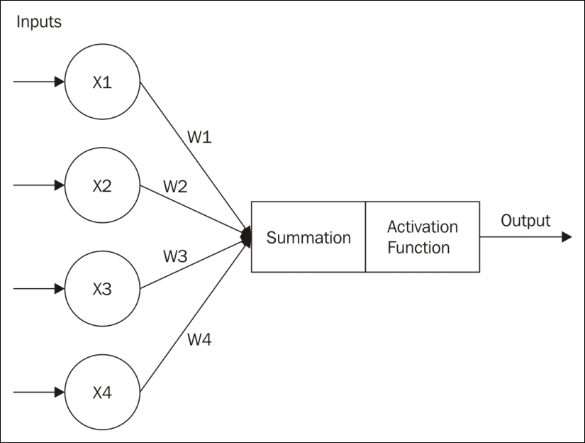
An artificial neuron is a node that has one or more inputs and a single output. Each input has a weight associated with it. By weighting inputs, we can amplify or de-amplify an input.
This is depicted in the following diagram, where the weights are summed and then sent to an Activation Function that determines the Output.
The neuron, and ultimately a collection of neurons, operate in one of two modes:
- Training mode - The neuron is trained to fire when a certain set of inputs are received
- Testing mode - Input is provided to the neuron, which responds as trained to a known set of inputs
A dataset is frequently split into two parts. A larger part is used to train a model. The second part is used to test and verify the model.
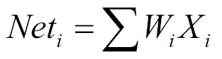
The output of a neuron is determined by the sum of the weighted inputs. Whether a neuron fires or not is determined by an activation function. There are several different types of activations functions, including:
- Step function - This linear function is computed using the summation of the weighted inputs as follows:
The f(Net) designates the output of a function. It is 1, if the Net input is greater than the activation threshold. When this happens the neuron fires. Otherwise it returns 0 and doesn't fire. The value is calculated based on all of the dendrite inputs.
- Sigmoid - This is a nonlinear function and is computed as follows:

As the neuron is trained, the weights with each input can be adjusted.
In contrast to the step function, the sigmoid function is non-linear. This better matches some problem domains. We will find the sigmoid function used in multi-layer neural networks.
There are three basic training approaches:
- Supervised learning - With supervised learning the model is trained with data that matches input sets to output values
- Unsupervised learning - In unsupervised learning, the data does not contain results, but the model is expected to determine relationships on its own
- Reinforcement learning - Similar to supervised learning, but a reward is provided for good results
These datasets differ in the information they contain. Supervised and reinforcement learning contain correct output for a set of input. The unsupervised learning does not contain correct results.
A neural network learns (at least with supervised learning) by feeding an input into a network and comparing the results, using the activation function, to the expected outcome. If they match, then the network has been trained correctly. If they don't match then the network is modified.
When we modify the weights we need to be careful not to change them too drastically. If the change is too large, then the results may change too much and we may miss the desired output. If the change is too little, then training the model will take too long. There are times when we may not want to change some weights.
A bias unit is a neuron that has a constant output. It is always one and is sometimes referred to as a fake node. This neuron is similar to an offset and is essential for most networks to function properly. You could compare the bias neuron to the y-intercept of a linear function in slope-intercept form. Just as adjusting the y-intercept value changes the location of the line, but not the shape/slope, the bias neuron can change the output values without adjusting the shape or function of the network. You can adjust the outputs to fit the particular needs of your problem.
Neural networks are usually created using a series of layers of neurons. There is typically an Input Layer, one or more middle layers (Hidden Layer), and an Output Layer.
The following is the depiction of a feedforward network:
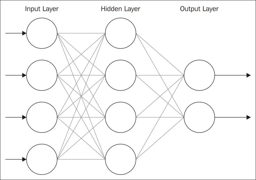
The number of nodes and layers will vary. A feedforward network moves the information forward. There are also feedback networks where information is passed backwards. Multiple hidden layers are needed to handle the more complicated processing required for most analysis.
We will discuss several architectures and algorithms related to different types of neural networks throughout this chapter. Due to the complexity and length of explanation required, we will only provide in-depth analysis of a few key network types. Specifically, we will demonstrate a simple neural network, MLPs, and Self-Organizing Maps (SOMs).
We will, however, provide an overview of many different options. The type of neural network and algorithm implementation appropriate for any particular model will depend upon the problem being addressed.
Static neural networks are ANNs that undergo a training or learning phase and then do not change when they are used. They differ from dynamic neural networks, which learn constantly and may undergo structural changes after the initial training period. Static neural networks are useful when the results of a model are relatively easy to reproduce or are more predictable. We will look at dynamic neural networks in a moment, but we will begin by creating our own basic static neural network.
Before we examine various libraries and tools available for constructing neural networks, we will implement our own basic neural network using standard Java libraries. The next example is an adaptation of work done by Jeff Heaton (http://www.informit.com/articles/article.aspx?p=30596). We will construct a feed-forward backpropagation neural network and train it to recognize the XOR operator pattern. Here is the basic truth table for XOR:
|
X |
Y |
Result |
|
|
|
|
|
|
|
|
|
|
|
|
|
|
|
|
This network needs only two input neurons and one output neuron corresponding to the X and Y input and the result. The number of input and output neurons needed for models is dependent upon the problem at hand. The number of hidden neurons is often the sum of the number of input and output neurons, but the exact number may need to be changed as training progresses.
We are going to demonstrate how to create and train the network next. We first provide the network with an input and observe the output. The output is compared to the expected output and then the weight matrix, called weightChanges, is adjusted. This adjustment ensures that the subsequent output will be closer to the expected output. This process is repeated until we are satisfied that the network can produce results significantly close enough to the expected output. In this example, we present the input and output as arrays of doubles where each input or output neuron is an element of the array.
First, we will create a SampleNeuralNetwork class to implement the network. Begin by adding the variables listed underneath to the class. We will discuss and demonstrate their purposes later in this section. Our class contains the following instance variables:
double errors; int inputNeurons; int outputNeurons; int hiddenNeurons; int totalNeurons; int weights; double learningRate; double outputResults[]; double resultsMatrix[]; double lastErrors[]; double changes[]; double thresholds[]; double weightChanges[]; double allThresholds[]; double threshChanges[]; double momentum; double errorChanges[];
Next, let's take a look at our constructor. We have four parameters, representing the number of inputs to our network, the number of neurons in hidden layers, the number of output neurons, and the rate and momentum at which we wish for learning to occur. The learningRate is a parameter that specifies the magnitude of changes in weight and bias during the training process. The momentum parameter specifies what fraction of a previous weight should be added to create a new weight. It is useful to prevent convergence at local minimums or saddle points. A high momentum increases the speed of convergence in a system, but can lead to an unstable system if it is too high. Both the momentum and learning rate should be values between 0 and 1:
public SampleNeuralNetwork(int inputCount,
int hiddenCount,
int outputCount,
double learnRate,
double momentum) {
...
}
Within our constructor we initialize all private instance variables. Notice that totalNeurons is set to the sum of all inputs, outputs, and hidden neurons. This sum is then used to set several other variables. Also notice that the weights variable is calculated by finding the product of the number of inputs and hidden neurons, the product of the hidden neurons and the outputs, and adding these two products together. This is then used to create new arrays of length weight:
learningRate = learnRate;
momentum = momentum;
inputNeurons = inputCount;
hiddenNeurons = hiddenCount;
outputNeurons = outputCount;
totalNeurons = inputCount + hiddenCount + outputCount;
weights = (inputCount * hiddenCount)
+ (hiddenCount * outputCount);
outputResults = new double[totalNeurons];
resultsMatrix = new double[weights];
weightChanges = new double[weights];
thresholds = new double[totalNeurons];
errorChanges = new double[totalNeurons];
lastErrors = new double[totalNeurons];
allThresholds = new double[totalNeurons];
changes = new double[weights];
threshChanges = new double[totalNeurons];
reset();
Notice that we call the reset method at the end of the constructor. This method resets the network to begin training with a random weight matrix. It initializes the thresholds and results matrices to random values. It also ensures that all matrices used for tracking changes are set back to zero. Using random values ensures that different results can be obtained:
public void reset() {
int loc;
for (loc = 0; loc < totalNeurons; loc++) {
thresholds[loc] = 0.5 - (Math.random());
threshChanges[loc] = 0;
allThresholds[loc] = 0;
}
for (loc = 0; loc < resultsMatrix.length; loc++) {
resultsMatrix[loc] = 0.5 - (Math.random());
weightChanges[loc] = 0;
changes[loc] = 0;
}
}
We also need a method called calcThreshold. The threshold value specifies how close a value has to be to the actual activation threshold before the neuron will fire. For example, a neuron may have an activation threshold of 1. The threshold value specifies whether a number such as 0.999 counts as 1. This method will be used in subsequent methods to calculate the thresholds for individual values:
public double threshold(double sum) {
return 1.0 / (1 + Math.exp(-1.0 * sum));
}
Next, we will add a method to calculate the output using a given set of inputs. Both our input parameter and the data returned by the method are arrays of double values. First, we need two position variables to use in our loops, loc and pos. We also want to keep track of our position within arrays based upon the number of input and hidden neurons. The index for our hidden neurons will start after our input neurons, so its position is the same as the number of input neurons. The position of our output neurons is the sum of our input neurons and hidden neurons. We also need to initialize our outputResults array:
public double[] calcOutput(double input[]) {
int loc, pos;
final int hiddenIndex = inputNeurons;
final int outIndex = inputNeurons + hiddenNeurons;
for (loc = 0; loc < inputNeurons; loc++) {
outputResults[loc] = input[loc];
}
...
}
Then we calculate outputs based upon our input neurons for the first layer of our network. Notice our use of the threshold method within this section. Before we can place our sum in the outputResults array, we need to utilize the threshold method:
int rLoc = 0;
for (loc = hiddenIndex; loc < outIndex; loc++) {
double sum = thresholds[loc];
for (pos = 0; pos < inputNeurons; pos++) {
sum += outputResults[pos] * resultsMatrix[rLoc++];
}
outputResults[loc] = threshold(sum);
}
Now we take into account our hidden neurons. Notice the process is similar to the previous section, but we are calculating outputs for the hidden layer rather than the input layer. At the end, we return our result. This result is in the form of an array of doubles containing the values of each output neuron. In our example, there is only one output neuron:
double result[] = new double[outputNeurons];
for (loc = outIndex; loc < totalNeurons; loc++) {
double sum = thresholds[loc];
for (pos = hiddenIndex; pos < outIndex; pos++) {
sum += outputResults[pos] * resultsMatrix[rLoc++];
}
outputResults[loc] = threshold(sum);
result[loc-outIndex] = outputResults[loc];
}
return result;
It is quite likely that the output does not match the expected output, given our XOR table. To handle this, we use error calculation methods to adjust the weights of our network to produce better output. The first method we will discuss is the calcError method. This method will be called every time a set of outputs is returned by the calcOutput method. It does not return data, but rather modifies arrays containing weight and threshold values. The method takes an array of doubles representing the ideal value for each output neuron. Notice we begin as we did in the calcOutput method and set up indexes to use throughout the method. Then we clear out any existing hidden layer errors:
public void calcError(double ideal[]) {
int loc, pos;
final int hiddenIndex = inputNeurons;
final int outputIndex = inputNeurons + hiddenNeurons;
for (loc = inputNeurons; loc < totalNeurons; loc++) {
lastErrors[loc] = 0;
}
Next we calculate the difference between our expected output and our actual output. This allows us to determine how to adjust the weights for further training. To do this, we loop through our arrays containing the expected outputs, ideal, and the actual outputs, outputResults. We also adjust our errors and change in errors in this section:
for (loc = outputIndex; loc < totalNeurons; loc++) {
lastErrors[loc] = ideal[loc - outputIndex] -
outputResults[loc];
errors += lastErrors[loc] * lastErrors[loc];
errorChanges[loc] = lastErrors[loc] * outputResults[loc]
*(1 - outputResults[loc]);
}
int locx = inputNeurons * hiddenNeurons;
for (loc = outputIndex; loc < totalNeurons; loc++) {
for (pos = hiddenIndex; pos < outputIndex; pos++) {
changes[locx] += errorChanges[loc] *
outputResults[pos];
lastErrors[pos] += resultsMatrix[locx] *
errorChanges[loc];
locx++;
}
allThresholds[loc] += errorChanges[loc];
}
Next we calculate and store the change in errors for each neuron. We use the lastErrors array to modify the errorChanges array, which contains total errors:
for (loc = hiddenIndex; loc < outputIndex; loc++) {
errorChanges[loc] = lastErrors[loc] *outputResults[loc]
* (1 - outputResults[loc]);
}We also fine tune our system by making changes to the allThresholds array. It is important to monitor the changes in errors and thresholds so the network can improve its ability to produce correct output:
locx = 0;
for (loc = hiddenIndex; loc < outputIndex; loc++) {
for (pos = 0; pos < hiddenIndex; pos++) {
changes[locx] += errorChanges[loc] *
outputResults[pos];
lastErrors[pos] += resultsMatrix[locx] *
errorChanges[loc];
locx++;
}
allThresholds[loc] += errorChanges[loc];
}
}
We have one other method used for calculating errors in our network. The getError method calculates the root mean square for our entire set of training data. This allows us to identify our average error rate for the data:
public double getError(int len) {
double err = Math.sqrt(errors / (len * outputNeurons));
errors = 0;
return err;
}
Now that we can initialize our network, compute outputs, and calculate errors, we are ready to train our network. We accomplish this through the use of the train method. This method makes adjustments first to the weights based upon the errors calculated in the previous method, and then adjusts the thresholds:
public void train() {
int loc;
for (loc = 0; loc < resultsMatrix.length; loc++) {
weightChanges[loc] = (learningRate * changes[loc]) +
(momentum * weightChanges[loc]);
resultsMatrix[loc] += weightChanges[loc];
changes[loc] = 0;
}
for (loc = inputNeurons; loc < totalNeurons; loc++) {
threshChanges[loc] = learningRate * allThresholds[loc] +
(momentum * threshChanges[loc]);
thresholds[loc] += threshChanges[loc];
allThresholds[loc] = 0;
}
}
Finally, we can create a new class to test our neural network. Within the main method of another class, add the following code to represent the XOR problem:
double xorIN[][] ={
{0.0,0.0},
{1.0,0.0},
{0.0,1.0},
{1.0,1.0}};
double xorEXPECTED[][] = { {0.0},{1.0},{1.0},{0.0}};
Next we want to create our new SampleNeuralNetwork object. In the following example, we have two input neurons, three hidden neurons, one output neuron (the XOR result), a learn rate of 0.7, and a momentum of 0.9. The number of hidden neurons is often best determined by trial and error. In subsequent executions, consider adjusting the values in this constructor and examine the difference in results:
SampleNeuralNetwork network = new
SampleNeuralNetwork(2,3,1,0.7,0.9);
We then repeatedly call our calcOutput, calcError, and train methods, in that order. This allows us to test our output, calculate the error rate, adjust our network weights, and then try again. Our network should display increasingly accurate results:
for (int runCnt=0;runCnt<10000;runCnt++) {
for (int loc=0;loc<xorIN.length;loc++) {
network.calcOutput(xorIN[loc]);
network.calcError(xorEXPECTED[loc]);
network.train();
}
System.out.println("Trial #" + runCnt + ",Error:" +
network.getError(xorIN.length));
}
Execute the application and notice that the error rate changes with each iteration of the loop. The acceptable error rate will depend upon the particular network and its purpose. The following is some sample output from the preceding code. For brevity we have included the first and the last training output. Notice that the error rate is initially above 50%, but falls to close to 1% by the last run:
Trial #0,Error:0.5338334002845255 Trial #1,Error:0.5233475199946769 Trial #2,Error:0.5229843653785426 Trial #3,Error:0.5226263062497853 Trial #4,Error:0.5226916275713371 ... Trial #994,Error:0.014457034704806316 Trial #995,Error:0.01444865096401158 Trial #996,Error:0.01444028142777395 Trial #997,Error:0.014431926056394229 Trial #998,Error:0.01442358481032747 Trial #999,Error:0.014415257650182488
In this example, we have used a small scale problem and we were able to train our network rather quickly. In a larger scale problem, we would start with a training set of data and then use additional datasets for further analysis. Because we really only have four inputs in this scenario, we will not test it with any additional data.
This example demonstrates some of the inner workings of a neural network, including details about how errors and output can be calculated. By exploring a relatively simple problem we are able to examine the mechanics of a neural network. In our next examples, however, we will use tools that hide these details from us, but allow us to conduct robust analysis.
A basic Java example
Before we examine various libraries and tools available for constructing neural networks, we will implement our own basic neural network using standard Java libraries. The next example is an adaptation of work done by Jeff Heaton (http://www.informit.com/articles/article.aspx?p=30596). We will construct a feed-forward backpropagation neural network and train it to recognize the XOR operator pattern. Here is the basic truth table for XOR:
|
X |
Y |
Result |
|
|
|
|
|
|
|
|
|
|
|
|
|
|
|
|
This network needs only two input neurons and one output neuron corresponding to the X and Y input and the result. The number of input and output neurons needed for models is dependent upon the problem at hand. The number of hidden neurons is often the sum of the number of input and output neurons, but the exact number may need to be changed as training progresses.
We are going to demonstrate how to create and train the network next. We first provide the network with an input and observe the output. The output is compared to the expected output and then the weight matrix, called weightChanges, is adjusted. This adjustment ensures that the subsequent output will be closer to the expected output. This process is repeated until we are satisfied that the network can produce results significantly close enough to the expected output. In this example, we present the input and output as arrays of doubles where each input or output neuron is an element of the array.
First, we will create a SampleNeuralNetwork class to implement the network. Begin by adding the variables listed underneath to the class. We will discuss and demonstrate their purposes later in this section. Our class contains the following instance variables:
double errors; int inputNeurons; int outputNeurons; int hiddenNeurons; int totalNeurons; int weights; double learningRate; double outputResults[]; double resultsMatrix[]; double lastErrors[]; double changes[]; double thresholds[]; double weightChanges[]; double allThresholds[]; double threshChanges[]; double momentum; double errorChanges[];
Next, let's take a look at our constructor. We have four parameters, representing the number of inputs to our network, the number of neurons in hidden layers, the number of output neurons, and the rate and momentum at which we wish for learning to occur. The learningRate is a parameter that specifies the magnitude of changes in weight and bias during the training process. The momentum parameter specifies what fraction of a previous weight should be added to create a new weight. It is useful to prevent convergence at local minimums or saddle points. A high momentum increases the speed of convergence in a system, but can lead to an unstable system if it is too high. Both the momentum and learning rate should be values between 0 and 1:
public SampleNeuralNetwork(int inputCount,
int hiddenCount,
int outputCount,
double learnRate,
double momentum) {
...
}
Within our constructor we initialize all private instance variables. Notice that totalNeurons is set to the sum of all inputs, outputs, and hidden neurons. This sum is then used to set several other variables. Also notice that the weights variable is calculated by finding the product of the number of inputs and hidden neurons, the product of the hidden neurons and the outputs, and adding these two products together. This is then used to create new arrays of length weight:
learningRate = learnRate;
momentum = momentum;
inputNeurons = inputCount;
hiddenNeurons = hiddenCount;
outputNeurons = outputCount;
totalNeurons = inputCount + hiddenCount + outputCount;
weights = (inputCount * hiddenCount)
+ (hiddenCount * outputCount);
outputResults = new double[totalNeurons];
resultsMatrix = new double[weights];
weightChanges = new double[weights];
thresholds = new double[totalNeurons];
errorChanges = new double[totalNeurons];
lastErrors = new double[totalNeurons];
allThresholds = new double[totalNeurons];
changes = new double[weights];
threshChanges = new double[totalNeurons];
reset();
Notice that we call the reset method at the end of the constructor. This method resets the network to begin training with a random weight matrix. It initializes the thresholds and results matrices to random values. It also ensures that all matrices used for tracking changes are set back to zero. Using random values ensures that different results can be obtained:
public void reset() {
int loc;
for (loc = 0; loc < totalNeurons; loc++) {
thresholds[loc] = 0.5 - (Math.random());
threshChanges[loc] = 0;
allThresholds[loc] = 0;
}
for (loc = 0; loc < resultsMatrix.length; loc++) {
resultsMatrix[loc] = 0.5 - (Math.random());
weightChanges[loc] = 0;
changes[loc] = 0;
}
}
We also need a method called calcThreshold. The threshold value specifies how close a value has to be to the actual activation threshold before the neuron will fire. For example, a neuron may have an activation threshold of 1. The threshold value specifies whether a number such as 0.999 counts as 1. This method will be used in subsequent methods to calculate the thresholds for individual values:
public double threshold(double sum) {
return 1.0 / (1 + Math.exp(-1.0 * sum));
}
Next, we will add a method to calculate the output using a given set of inputs. Both our input parameter and the data returned by the method are arrays of double values. First, we need two position variables to use in our loops, loc and pos. We also want to keep track of our position within arrays based upon the number of input and hidden neurons. The index for our hidden neurons will start after our input neurons, so its position is the same as the number of input neurons. The position of our output neurons is the sum of our input neurons and hidden neurons. We also need to initialize our outputResults array:
public double[] calcOutput(double input[]) {
int loc, pos;
final int hiddenIndex = inputNeurons;
final int outIndex = inputNeurons + hiddenNeurons;
for (loc = 0; loc < inputNeurons; loc++) {
outputResults[loc] = input[loc];
}
...
}
Then we calculate outputs based upon our input neurons for the first layer of our network. Notice our use of the threshold method within this section. Before we can place our sum in the outputResults array, we need to utilize the threshold method:
int rLoc = 0;
for (loc = hiddenIndex; loc < outIndex; loc++) {
double sum = thresholds[loc];
for (pos = 0; pos < inputNeurons; pos++) {
sum += outputResults[pos] * resultsMatrix[rLoc++];
}
outputResults[loc] = threshold(sum);
}
Now we take into account our hidden neurons. Notice the process is similar to the previous section, but we are calculating outputs for the hidden layer rather than the input layer. At the end, we return our result. This result is in the form of an array of doubles containing the values of each output neuron. In our example, there is only one output neuron:
double result[] = new double[outputNeurons];
for (loc = outIndex; loc < totalNeurons; loc++) {
double sum = thresholds[loc];
for (pos = hiddenIndex; pos < outIndex; pos++) {
sum += outputResults[pos] * resultsMatrix[rLoc++];
}
outputResults[loc] = threshold(sum);
result[loc-outIndex] = outputResults[loc];
}
return result;
It is quite likely that the output does not match the expected output, given our XOR table. To handle this, we use error calculation methods to adjust the weights of our network to produce better output. The first method we will discuss is the calcError method. This method will be called every time a set of outputs is returned by the calcOutput method. It does not return data, but rather modifies arrays containing weight and threshold values. The method takes an array of doubles representing the ideal value for each output neuron. Notice we begin as we did in the calcOutput method and set up indexes to use throughout the method. Then we clear out any existing hidden layer errors:
public void calcError(double ideal[]) {
int loc, pos;
final int hiddenIndex = inputNeurons;
final int outputIndex = inputNeurons + hiddenNeurons;
for (loc = inputNeurons; loc < totalNeurons; loc++) {
lastErrors[loc] = 0;
}
Next we calculate the difference between our expected output and our actual output. This allows us to determine how to adjust the weights for further training. To do this, we loop through our arrays containing the expected outputs, ideal, and the actual outputs, outputResults. We also adjust our errors and change in errors in this section:
for (loc = outputIndex; loc < totalNeurons; loc++) {
lastErrors[loc] = ideal[loc - outputIndex] -
outputResults[loc];
errors += lastErrors[loc] * lastErrors[loc];
errorChanges[loc] = lastErrors[loc] * outputResults[loc]
*(1 - outputResults[loc]);
}
int locx = inputNeurons * hiddenNeurons;
for (loc = outputIndex; loc < totalNeurons; loc++) {
for (pos = hiddenIndex; pos < outputIndex; pos++) {
changes[locx] += errorChanges[loc] *
outputResults[pos];
lastErrors[pos] += resultsMatrix[locx] *
errorChanges[loc];
locx++;
}
allThresholds[loc] += errorChanges[loc];
}
Next we calculate and store the change in errors for each neuron. We use the lastErrors array to modify the errorChanges array, which contains total errors:
for (loc = hiddenIndex; loc < outputIndex; loc++) {
errorChanges[loc] = lastErrors[loc] *outputResults[loc]
* (1 - outputResults[loc]);
}We also fine tune our system by making changes to the allThresholds array. It is important to monitor the changes in errors and thresholds so the network can improve its ability to produce correct output:
locx = 0;
for (loc = hiddenIndex; loc < outputIndex; loc++) {
for (pos = 0; pos < hiddenIndex; pos++) {
changes[locx] += errorChanges[loc] *
outputResults[pos];
lastErrors[pos] += resultsMatrix[locx] *
errorChanges[loc];
locx++;
}
allThresholds[loc] += errorChanges[loc];
}
}
We have one other method used for calculating errors in our network. The getError method calculates the root mean square for our entire set of training data. This allows us to identify our average error rate for the data:
public double getError(int len) {
double err = Math.sqrt(errors / (len * outputNeurons));
errors = 0;
return err;
}
Now that we can initialize our network, compute outputs, and calculate errors, we are ready to train our network. We accomplish this through the use of the train method. This method makes adjustments first to the weights based upon the errors calculated in the previous method, and then adjusts the thresholds:
public void train() {
int loc;
for (loc = 0; loc < resultsMatrix.length; loc++) {
weightChanges[loc] = (learningRate * changes[loc]) +
(momentum * weightChanges[loc]);
resultsMatrix[loc] += weightChanges[loc];
changes[loc] = 0;
}
for (loc = inputNeurons; loc < totalNeurons; loc++) {
threshChanges[loc] = learningRate * allThresholds[loc] +
(momentum * threshChanges[loc]);
thresholds[loc] += threshChanges[loc];
allThresholds[loc] = 0;
}
}
Finally, we can create a new class to test our neural network. Within the main method of another class, add the following code to represent the XOR problem:
double xorIN[][] ={
{0.0,0.0},
{1.0,0.0},
{0.0,1.0},
{1.0,1.0}};
double xorEXPECTED[][] = { {0.0},{1.0},{1.0},{0.0}};
Next we want to create our new SampleNeuralNetwork object. In the following example, we have two input neurons, three hidden neurons, one output neuron (the XOR result), a learn rate of 0.7, and a momentum of 0.9. The number of hidden neurons is often best determined by trial and error. In subsequent executions, consider adjusting the values in this constructor and examine the difference in results:
SampleNeuralNetwork network = new
SampleNeuralNetwork(2,3,1,0.7,0.9);
We then repeatedly call our calcOutput, calcError, and train methods, in that order. This allows us to test our output, calculate the error rate, adjust our network weights, and then try again. Our network should display increasingly accurate results:
for (int runCnt=0;runCnt<10000;runCnt++) {
for (int loc=0;loc<xorIN.length;loc++) {
network.calcOutput(xorIN[loc]);
network.calcError(xorEXPECTED[loc]);
network.train();
}
System.out.println("Trial #" + runCnt + ",Error:" +
network.getError(xorIN.length));
}
Execute the application and notice that the error rate changes with each iteration of the loop. The acceptable error rate will depend upon the particular network and its purpose. The following is some sample output from the preceding code. For brevity we have included the first and the last training output. Notice that the error rate is initially above 50%, but falls to close to 1% by the last run:
Trial #0,Error:0.5338334002845255 Trial #1,Error:0.5233475199946769 Trial #2,Error:0.5229843653785426 Trial #3,Error:0.5226263062497853 Trial #4,Error:0.5226916275713371 ... Trial #994,Error:0.014457034704806316 Trial #995,Error:0.01444865096401158 Trial #996,Error:0.01444028142777395 Trial #997,Error:0.014431926056394229 Trial #998,Error:0.01442358481032747 Trial #999,Error:0.014415257650182488
In this example, we have used a small scale problem and we were able to train our network rather quickly. In a larger scale problem, we would start with a training set of data and then use additional datasets for further analysis. Because we really only have four inputs in this scenario, we will not test it with any additional data.
This example demonstrates some of the inner workings of a neural network, including details about how errors and output can be calculated. By exploring a relatively simple problem we are able to examine the mechanics of a neural network. In our next examples, however, we will use tools that hide these details from us, but allow us to conduct robust analysis.
Dynamic neural networks differ from static networks in that they continue learning after the training phase. They can make adjustments to their structure independently of external modification. A feedforward neural network (FNN) is one of the earliest and simplest dynamic neural networks. This type of network, as its name implies, only feeds information forward and does not form any cycles. This type of network formed the foundation for much of the later work in dynamic ANNs. We will show in-depth examples of two types of dynamic networks in this section, MLP networks and SOMs.
A MLP network is a FNN with multiple layers. The network uses supervised learning with backpropagation where feedback is sent to early layers to assist in the learning process. Some of the neurons use a nonlinear activation function mimicking biological neurons. Every nodes of one layer is fully connected to the following layer.
We will use a dataset called dermatology.arff that can be downloaded from http://repository.seasr.org/Datasets/UCI/arff/. This dataset contains 366 instances used to diagnosis erythemato-squamous diseases. It uses 34 attributes to classify the disease into one of five different categories. The following is a sample instance:
2,2,0,3,0,0,0,0,1,0,0,0,0,0,0,3,2,0,0,0,0,0,0,0,0,0,0,3,0,0,0,1,0,55,2
The last field represents the disease category. This dataset has been partitioned into two files: dermatologyTrainingSet.arff and dermatologyTestingSet.arff. The training set uses the first 80% (292 instances) of the original set and ends with line 456. The testing set is the last 20% (74 instances) and starts with line 457 of the original set (lines 457-530).
Before we can make any predictions, it is necessary that we train the model on a representative set of data. We will use the Weka class, MultilayerPerceptron, for training and eventually to make predictions. First, we declare strings for the training and testing of filenames and the corresponding FileReader instances for them. The instances are created and the last field is specified as the field to use for classification:
String trainingFileName = "dermatologyTrainingSet.arff";
String testingFileName = "dermatologyTestingSet.arff";
try (FileReader trainingReader = new FileReader(trainingFileName);
FileReader testingReader =
new FileReader(testingFileName)) {
Instances trainingInstances = new Instances(trainingReader);
trainingInstances.setClassIndex(
trainingInstances.numAttributes() - 1);
Instances testingInstances = new Instances(testingReader);
testingInstances.setClassIndex(
testingInstances.numAttributes() - 1);
...
} catch (Exception ex) {
// Handle exceptions
}
An instance of the MultilayerPerceptron class is then created:
MultilayerPerceptron mlp = new MultilayerPerceptron();
There are several model parameters that we can set, as shown here:
|
Parameter |
Method |
Description |
|
Learning rate |
|
Affects the training speed |
|
Momentum |
|
Affects the training speed |
|
Training time |
|
The number of training epochs used to train the model |
|
Hidden layers |
|
The number of hidden layers and perceptrons to use |
As mentioned previously, the learning rate will affect the speed in which your model is trained. A large value can increase the training speed. If the learning rate is too small, then the training time may take too long. If the learning rate is too large, then the model may move past a local minimum and become divergent. That is, if the increase is too large, we might skip over a meaningful value. You can think of this a graph where a small dip in a plot along the Y axis is missed because we incremented our X value too much.
Momentum also affects the training speed by effectively increasing the rate of learning. It is used in addition to the learning rate to add momentum to the search for the optimal value. In the case of a local minimum, the momentum helps get out of the minimum in its quest for a global minimum.
When the model is learning it performs operations iteratively. The term, epoch is used to refer to the number of iterations. Hopefully, the total error encounter with each epoch will decrease to a point where further epochs are not useful. It is ideal to avoid too many epochs.
A neural network will have one or more hidden layers. Each of these layers will have a specific number of perceptrons. The setHiddenLayers method specifies the number of layers and perceptrons using a string. For example, 3,5 would specify two hidden layers with three and five perceptrons per layer, respectively.
For this example, we will use the following values:
mlp.setLearningRate(0.1);
mlp.setMomentum(0.2);
mlp.setTrainingTime(2000);
mlp.setHiddenLayers("3");
The buildClassifier method uses the training data to build the model:
mlp.buildClassifier(trainingInstances);
The next step is to evaluate the model. The Evaluation class is used for this purpose. Its constructor takes the training set as input and the evaluateModel method performs the actual evaluation. The following code illustrates this using the testing dataset:
Evaluation evaluation = new Evaluation(trainingInstances); evaluation.evaluateModel(mlp, testingInstances);
One simple way of displaying the results of the evaluation is using the toSummaryString method:
System.out.println(evaluation.toSummaryString());
This will display the following output:
Correctly Classified Instances 73 98.6486 % Incorrectly Classified Instances 1 1.3514 % Kappa statistic 0.9824 Mean absolute error 0.0177 Root mean squared error 0.076 Relative absolute error 6.6173 % Root relative squared error 20.7173 % Coverage of cases (0.95 level) 98.6486 % Mean rel. region size (0.95 level) 18.018 % Total Number of Instances 74
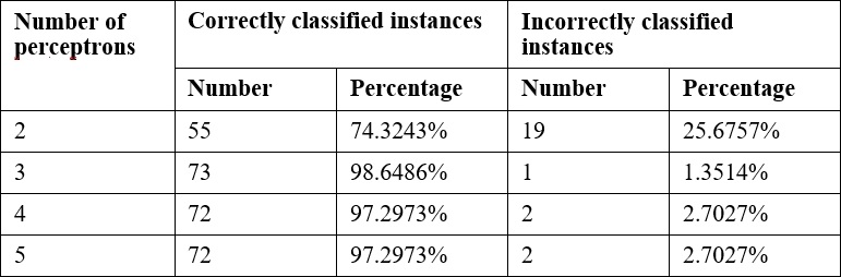
Frequently, it will be necessary to experiment with these parameters to get the best results. The following are the results of varying the number of perceptrons:
Once we have a model trained, we can use it to evaluate other data. In the previous testing dataset there was one instance which failed. In the following code sequence, this instance is identified and the predicted and actual results are displayed.
Each instance of the testing dataset is used as input to the classifyInstance method. This method tries to predict the correct result. This result is compared to the last field of the instance that contains the actual value. For mismatches, the predicted and actual values are displayed:
for (int i = 0; i < testingInstances.numInstances(); i++) {
double result = mlp.classifyInstance(
testingInstances.instance(i));
if (result != testingInstances
.instance(i)
.value(testingInstances.numAttributes() - 1)) {
out.println("Classify result: " + result
+ " Correct: " + testingInstances.instance(i)
.value(testingInstances.numAttributes() - 1));
...
}
}
For the testing set we get the following output:
Classify result: 1.0 Correct: 3.0
We can get the likelihood of the prediction being correct using the MultilayerPerceptron class' distributionForInstance method. Place the following code into the previous loop. It will capture the incorrect instance, which is easier than instantiating an instance based on the 34 attributes used by the dataset. The distributionForInstance method takes this instance and returns a two element array of doubles. The first element is the probability of the result being positive and the second is the probability of it being negative:
Instance incorrectInstance = testingInstances.instance(i);
incorrectInstance.setDataset(trainingInstances);
double[] distribution = mlp.distributionForInstance(incorrectInstance);
out.println("Probability of being positive: " + distribution[0]);
out.println("Probability of being negative: " + distribution[1]); The output for this instance is as follows:
Probability of being positive: 0.00350515156929017 Probability of being negative: 0.9683660500711128
This can provide a more quantitative feel for the reliability of the prediction.
We can also save and retrieve a model for later use. To save the model, build the model and then use the SerializationHelper class' static method write, as shown in the following code snippet. The first argument is the name of the file to hold the model:
SerializationHelper.write("mlpModel", mlp);
To retrieve the model, use the corresponding read method as shown here:
mlp = (MultilayerPerceptron)SerializationHelper.read("mlpModel");
Next, we will learn how to use another useful neural network approach, SOMs.
Learning Vector Quantization (LVQ) is another special type of a dynamic ANN. SOMs, which we will discuss in a moment, are a by-product of LVQ networks. This type of network implements a competitive type of algorithm in which the winning neuron gains the weight. These types of networks are used in many different applications and are considered to be more natural and intuitive than some other ANNs. In particular, LVQ is effective for classification of text-based data.
The basic algorithm begins by setting the number of neurons, the weight for each neuron, how fast the neurons can learn, and a list of input vectors. In this context, a vector is similar to a vector in physics and represents the values provided to the input layer neurons. As the network is trained, a vector is used as input, a winning neuron is selected, and the weight of the winning neuron is updated. This model is iterative and will continue to run until a solution is found.
SOMs is a technique that takes multidimensional data and reducing it to one or two dimensions. This compression technique is called vector quantization. The technique usually involves a visual component that allows a human to better see how the data has been categorized. SOM learns without supervision.
The SOM is good for finding clusters, which is not to be confused with classification. With classification we are interested in finding the best fit for a data instance among predefined categories. With clustering we are interested in grouping instances where the categories are unknown.
A SOM uses a lattice of neurons, usually a two-dimensional array or a hexagonal grid, representing neurons that are assigned weights. The input sources are connected to each of these neurons. The technique then adjusts the weights assigned to each lattice member through several iterations until the best fit is found. When finished, the lattice members will have grouped the input dataset into categories. The SOM results can be viewed to identify categories and map new input to one of the identified categories.
We will use the Weka to demonstrate SOM. However, it is does not come installed with standard Weka. Instead, we will need to download a set of Weka classification algorithms from https://sourceforge.net/projects/wekaclassalgos/files/ and the actual SOM class from http://www.cis.hut.fi/research/som_pak/. The classification algorithms include support for LVQ. More details about the classification algorithms can be found at http://wekaclassalgos.sourceforge.net/.
To use the SOM class, called SelfOrganizingMap, the source code needs to be in your project. The Javadoc for this class is found at http://jsalatas.ictpro.gr/weka/doc/SelfOrganizingMap/.
We start with the creation of an instance of the SelfOrganizingMap class. This is followed by code to read in data and create an Instances object to hold the data. In this example, we will use the iris.arff file, which can be found in the Weka data directory. Notice that once the Instances object is created we do not specify the class index as we did with previous Weka examples since SOM uses unsupervised learning:
SelfOrganizingMap som = new SelfOrganizingMap();
String trainingFileName = "iris.arff";
try (FileReader trainingReader =
new FileReader(trainingFileName)) {
Instances trainingInstances = new Instances(trainingReader);
...
} catch (IOException ex) {
// Handle exceptions
} catch (Exception ex) {
// Handle exceptions
}The buildClusterer method will execute the SOM algorithm using the training dataset:
som.buildClusterer(trainingInstances);
We can now display the results of the operation as follows:
out.println(som.toString());
The iris dataset uses five attributes: sepallength, sepalwidth, petallength, petalwidth, and class. The first four attributes are numeric and the fifth has three possible values: Iris-setosa, Iris-versicolor, and Iris-virginica. The first part of the abbreviated output that follows identified four clusters and the number of instances in each cluster. This is followed by statistics for each of the attributes:
Self Organized Map ================== Number of clusters: 4 Cluster Attribute 0 1 2 3 (50) (42) (29) (29) ============================================== sepallength value 5.0036 6.2365 5.5823 6.9513 min 4.3 5.6 4.9 6.2 max 5.8 7 6.3 7.9 mean 5.006 6.25 5.5828 6.9586 std. dev. 0.3525 0.3536 0.3675 0.5046 ... class value 0 1.5048 1.0787 2 min 0 1 1 2 max 0 2 2 2 mean 0 1.4524 1.069 2 std. dev. 0 0.5038 0.2579 0
These statistics can provide insight into the dataset. If we are interested in determining which dataset instance is found in a cluster, we can use the getClusterInstances method to return the array that groups the instances by cluster. As shown next, this method is used to list the instance by cluster:
Instances[] clusters = som.getClusterInstances();
int index = 0;
for (Instances instances : clusters) {
out.println("-------Custer " + index);
for (Instance instance : instances) {
out.println(instance);
}
out.println();
index++;
}
As we can see with the abbreviated output of this sequence, different iris classes are grouped into the different clusters:
-------Custer 0 5.1,3.5,1.4,0.2,Iris-setosa 4.9,3,1.4,0.2,Iris-setosa 4.7,3.2,1.3,0.2,Iris-setosa 4.6,3.1,1.5,0.2,Iris-setosa ... 5.3,3.7,1.5,0.2,Iris-setosa 5,3.3,1.4,0.2,Iris-setosa -------Custer 1 7,3.2,4.7,1.4,Iris-versicolor 6.4,3.2,4.5,1.5,Iris-versicolor 6.9,3.1,4.9,1.5,Iris-versicolor ... 6.5,3,5.2,2,Iris-virginica 5.9,3,5.1,1.8,Iris-virginica -------Custer 2 5.5,2.3,4,1.3,Iris-versicolor 5.7,2.8,4.5,1.3,Iris-versicolor 4.9,2.4,3.3,1,Iris-versicolor ... 4.9,2.5,4.5,1.7,Iris-virginica 6,2.2,5,1.5,Iris-virginica -------Custer 3 6.3,3.3,6,2.5,Iris-virginica 7.1,3,5.9,2.1,Iris-virginica 6.5,3,5.8,2.2,Iris-virginica ...
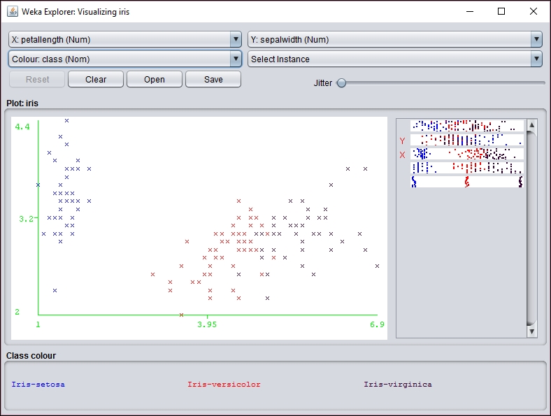
The cluster results can be displayed visually using the Weka GUI interface. In the following screenshot, we have used the Weka Workbench to analyze and visualize the result of the SOM analysis:
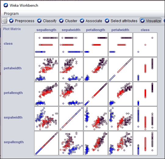
An individual section of the graph can be selected, customized, and analyzed as follows:
However, before you can use the SOM class, the WekaPackageManager must be used to add the SOM package to Weka. This process is discussed at https://weka.wikispaces.com/How+do+I+use+the+package+manager%3F.
If a new instance needs to be mapped to a cluster, the distributionForInstance method can be used as illustrated in Predicting other values section.
Multilayer perceptron networks
A MLP network is a FNN with multiple layers. The network uses supervised learning with backpropagation where feedback is sent to early layers to assist in the learning process. Some of the neurons use a nonlinear activation function mimicking biological neurons. Every nodes of one layer is fully connected to the following layer.
We will use a dataset called dermatology.arff that can be downloaded from http://repository.seasr.org/Datasets/UCI/arff/. This dataset contains 366 instances used to diagnosis erythemato-squamous diseases. It uses 34 attributes to classify the disease into one of five different categories. The following is a sample instance:
2,2,0,3,0,0,0,0,1,0,0,0,0,0,0,3,2,0,0,0,0,0,0,0,0,0,0,3,0,0,0,1,0,55,2
The last field represents the disease category. This dataset has been partitioned into two files: dermatologyTrainingSet.arff and dermatologyTestingSet.arff. The training set uses the first 80% (292 instances) of the original set and ends with line 456. The testing set is the last 20% (74 instances) and starts with line 457 of the original set (lines 457-530).
Before we can make any predictions, it is necessary that we train the model on a representative set of data. We will use the Weka class, MultilayerPerceptron, for training and eventually to make predictions. First, we declare strings for the training and testing of filenames and the corresponding FileReader instances for them. The instances are created and the last field is specified as the field to use for classification:
String trainingFileName = "dermatologyTrainingSet.arff";
String testingFileName = "dermatologyTestingSet.arff";
try (FileReader trainingReader = new FileReader(trainingFileName);
FileReader testingReader =
new FileReader(testingFileName)) {
Instances trainingInstances = new Instances(trainingReader);
trainingInstances.setClassIndex(
trainingInstances.numAttributes() - 1);
Instances testingInstances = new Instances(testingReader);
testingInstances.setClassIndex(
testingInstances.numAttributes() - 1);
...
} catch (Exception ex) {
// Handle exceptions
}
An instance of the MultilayerPerceptron class is then created:
MultilayerPerceptron mlp = new MultilayerPerceptron();
There are several model parameters that we can set, as shown here:
|
Parameter |
Method |
Description |
|
Learning rate |
|
Affects the training speed |
|
Momentum |
|
Affects the training speed |
|
Training time |
|
The number of training epochs used to train the model |
|
Hidden layers |
|
The number of hidden layers and perceptrons to use |
As mentioned previously, the learning rate will affect the speed in which your model is trained. A large value can increase the training speed. If the learning rate is too small, then the training time may take too long. If the learning rate is too large, then the model may move past a local minimum and become divergent. That is, if the increase is too large, we might skip over a meaningful value. You can think of this a graph where a small dip in a plot along the Y axis is missed because we incremented our X value too much.
Momentum also affects the training speed by effectively increasing the rate of learning. It is used in addition to the learning rate to add momentum to the search for the optimal value. In the case of a local minimum, the momentum helps get out of the minimum in its quest for a global minimum.
When the model is learning it performs operations iteratively. The term, epoch is used to refer to the number of iterations. Hopefully, the total error encounter with each epoch will decrease to a point where further epochs are not useful. It is ideal to avoid too many epochs.
A neural network will have one or more hidden layers. Each of these layers will have a specific number of perceptrons. The setHiddenLayers method specifies the number of layers and perceptrons using a string. For example, 3,5 would specify two hidden layers with three and five perceptrons per layer, respectively.
For this example, we will use the following values:
mlp.setLearningRate(0.1);
mlp.setMomentum(0.2);
mlp.setTrainingTime(2000);
mlp.setHiddenLayers("3");
The buildClassifier method uses the training data to build the model:
mlp.buildClassifier(trainingInstances);
The next step is to evaluate the model. The Evaluation class is used for this purpose. Its constructor takes the training set as input and the evaluateModel method performs the actual evaluation. The following code illustrates this using the testing dataset:
Evaluation evaluation = new Evaluation(trainingInstances); evaluation.evaluateModel(mlp, testingInstances);
One simple way of displaying the results of the evaluation is using the toSummaryString method:
System.out.println(evaluation.toSummaryString());
This will display the following output:
Correctly Classified Instances 73 98.6486 % Incorrectly Classified Instances 1 1.3514 % Kappa statistic 0.9824 Mean absolute error 0.0177 Root mean squared error 0.076 Relative absolute error 6.6173 % Root relative squared error 20.7173 % Coverage of cases (0.95 level) 98.6486 % Mean rel. region size (0.95 level) 18.018 % Total Number of Instances 74
Frequently, it will be necessary to experiment with these parameters to get the best results. The following are the results of varying the number of perceptrons:
Once we have a model trained, we can use it to evaluate other data. In the previous testing dataset there was one instance which failed. In the following code sequence, this instance is identified and the predicted and actual results are displayed.
Each instance of the testing dataset is used as input to the classifyInstance method. This method tries to predict the correct result. This result is compared to the last field of the instance that contains the actual value. For mismatches, the predicted and actual values are displayed:
for (int i = 0; i < testingInstances.numInstances(); i++) {
double result = mlp.classifyInstance(
testingInstances.instance(i));
if (result != testingInstances
.instance(i)
.value(testingInstances.numAttributes() - 1)) {
out.println("Classify result: " + result
+ " Correct: " + testingInstances.instance(i)
.value(testingInstances.numAttributes() - 1));
...
}
}
For the testing set we get the following output:
Classify result: 1.0 Correct: 3.0
We can get the likelihood of the prediction being correct using the MultilayerPerceptron class' distributionForInstance method. Place the following code into the previous loop. It will capture the incorrect instance, which is easier than instantiating an instance based on the 34 attributes used by the dataset. The distributionForInstance method takes this instance and returns a two element array of doubles. The first element is the probability of the result being positive and the second is the probability of it being negative:
Instance incorrectInstance = testingInstances.instance(i);
incorrectInstance.setDataset(trainingInstances);
double[] distribution = mlp.distributionForInstance(incorrectInstance);
out.println("Probability of being positive: " + distribution[0]);
out.println("Probability of being negative: " + distribution[1]); The output for this instance is as follows:
Probability of being positive: 0.00350515156929017 Probability of being negative: 0.9683660500711128
This can provide a more quantitative feel for the reliability of the prediction.
We can also save and retrieve a model for later use. To save the model, build the model and then use the SerializationHelper class' static method write, as shown in the following code snippet. The first argument is the name of the file to hold the model:
SerializationHelper.write("mlpModel", mlp);
To retrieve the model, use the corresponding read method as shown here:
mlp = (MultilayerPerceptron)SerializationHelper.read("mlpModel");
Next, we will learn how to use another useful neural network approach, SOMs.
Learning Vector Quantization (LVQ) is another special type of a dynamic ANN. SOMs, which we will discuss in a moment, are a by-product of LVQ networks. This type of network implements a competitive type of algorithm in which the winning neuron gains the weight. These types of networks are used in many different applications and are considered to be more natural and intuitive than some other ANNs. In particular, LVQ is effective for classification of text-based data.
The basic algorithm begins by setting the number of neurons, the weight for each neuron, how fast the neurons can learn, and a list of input vectors. In this context, a vector is similar to a vector in physics and represents the values provided to the input layer neurons. As the network is trained, a vector is used as input, a winning neuron is selected, and the weight of the winning neuron is updated. This model is iterative and will continue to run until a solution is found.
SOMs is a technique that takes multidimensional data and reducing it to one or two dimensions. This compression technique is called vector quantization. The technique usually involves a visual component that allows a human to better see how the data has been categorized. SOM learns without supervision.
The SOM is good for finding clusters, which is not to be confused with classification. With classification we are interested in finding the best fit for a data instance among predefined categories. With clustering we are interested in grouping instances where the categories are unknown.
A SOM uses a lattice of neurons, usually a two-dimensional array or a hexagonal grid, representing neurons that are assigned weights. The input sources are connected to each of these neurons. The technique then adjusts the weights assigned to each lattice member through several iterations until the best fit is found. When finished, the lattice members will have grouped the input dataset into categories. The SOM results can be viewed to identify categories and map new input to one of the identified categories.
We will use the Weka to demonstrate SOM. However, it is does not come installed with standard Weka. Instead, we will need to download a set of Weka classification algorithms from https://sourceforge.net/projects/wekaclassalgos/files/ and the actual SOM class from http://www.cis.hut.fi/research/som_pak/. The classification algorithms include support for LVQ. More details about the classification algorithms can be found at http://wekaclassalgos.sourceforge.net/.
To use the SOM class, called SelfOrganizingMap, the source code needs to be in your project. The Javadoc for this class is found at http://jsalatas.ictpro.gr/weka/doc/SelfOrganizingMap/.
We start with the creation of an instance of the SelfOrganizingMap class. This is followed by code to read in data and create an Instances object to hold the data. In this example, we will use the iris.arff file, which can be found in the Weka data directory. Notice that once the Instances object is created we do not specify the class index as we did with previous Weka examples since SOM uses unsupervised learning:
SelfOrganizingMap som = new SelfOrganizingMap();
String trainingFileName = "iris.arff";
try (FileReader trainingReader =
new FileReader(trainingFileName)) {
Instances trainingInstances = new Instances(trainingReader);
...
} catch (IOException ex) {
// Handle exceptions
} catch (Exception ex) {
// Handle exceptions
}The buildClusterer method will execute the SOM algorithm using the training dataset:
som.buildClusterer(trainingInstances);
We can now display the results of the operation as follows:
out.println(som.toString());
The iris dataset uses five attributes: sepallength, sepalwidth, petallength, petalwidth, and class. The first four attributes are numeric and the fifth has three possible values: Iris-setosa, Iris-versicolor, and Iris-virginica. The first part of the abbreviated output that follows identified four clusters and the number of instances in each cluster. This is followed by statistics for each of the attributes:
Self Organized Map ================== Number of clusters: 4 Cluster Attribute 0 1 2 3 (50) (42) (29) (29) ============================================== sepallength value 5.0036 6.2365 5.5823 6.9513 min 4.3 5.6 4.9 6.2 max 5.8 7 6.3 7.9 mean 5.006 6.25 5.5828 6.9586 std. dev. 0.3525 0.3536 0.3675 0.5046 ... class value 0 1.5048 1.0787 2 min 0 1 1 2 max 0 2 2 2 mean 0 1.4524 1.069 2 std. dev. 0 0.5038 0.2579 0
These statistics can provide insight into the dataset. If we are interested in determining which dataset instance is found in a cluster, we can use the getClusterInstances method to return the array that groups the instances by cluster. As shown next, this method is used to list the instance by cluster:
Instances[] clusters = som.getClusterInstances();
int index = 0;
for (Instances instances : clusters) {
out.println("-------Custer " + index);
for (Instance instance : instances) {
out.println(instance);
}
out.println();
index++;
}
As we can see with the abbreviated output of this sequence, different iris classes are grouped into the different clusters:
-------Custer 0 5.1,3.5,1.4,0.2,Iris-setosa 4.9,3,1.4,0.2,Iris-setosa 4.7,3.2,1.3,0.2,Iris-setosa 4.6,3.1,1.5,0.2,Iris-setosa ... 5.3,3.7,1.5,0.2,Iris-setosa 5,3.3,1.4,0.2,Iris-setosa -------Custer 1 7,3.2,4.7,1.4,Iris-versicolor 6.4,3.2,4.5,1.5,Iris-versicolor 6.9,3.1,4.9,1.5,Iris-versicolor ... 6.5,3,5.2,2,Iris-virginica 5.9,3,5.1,1.8,Iris-virginica -------Custer 2 5.5,2.3,4,1.3,Iris-versicolor 5.7,2.8,4.5,1.3,Iris-versicolor 4.9,2.4,3.3,1,Iris-versicolor ... 4.9,2.5,4.5,1.7,Iris-virginica 6,2.2,5,1.5,Iris-virginica -------Custer 3 6.3,3.3,6,2.5,Iris-virginica 7.1,3,5.9,2.1,Iris-virginica 6.5,3,5.8,2.2,Iris-virginica ...
The cluster results can be displayed visually using the Weka GUI interface. In the following screenshot, we have used the Weka Workbench to analyze and visualize the result of the SOM analysis:
An individual section of the graph can be selected, customized, and analyzed as follows:
However, before you can use the SOM class, the WekaPackageManager must be used to add the SOM package to Weka. This process is discussed at https://weka.wikispaces.com/How+do+I+use+the+package+manager%3F.
If a new instance needs to be mapped to a cluster, the distributionForInstance method can be used as illustrated in Predicting other values section.
Building the model
Before we can make any predictions, it is necessary that we train the model on a representative set of data. We will use the Weka class, MultilayerPerceptron, for training and eventually to make predictions. First, we declare strings for the training and testing of filenames and the corresponding FileReader instances for them. The instances are created and the last field is specified as the field to use for classification:
String trainingFileName = "dermatologyTrainingSet.arff";
String testingFileName = "dermatologyTestingSet.arff";
try (FileReader trainingReader = new FileReader(trainingFileName);
FileReader testingReader =
new FileReader(testingFileName)) {
Instances trainingInstances = new Instances(trainingReader);
trainingInstances.setClassIndex(
trainingInstances.numAttributes() - 1);
Instances testingInstances = new Instances(testingReader);
testingInstances.setClassIndex(
testingInstances.numAttributes() - 1);
...
} catch (Exception ex) {
// Handle exceptions
}
An instance of the MultilayerPerceptron class is then created:
MultilayerPerceptron mlp = new MultilayerPerceptron();
There are several model parameters that we can set, as shown here:
|
Parameter |
Method |
Description |
|
Learning rate |
|
Affects the training speed |
|
Momentum |
|
Affects the training speed |
|
Training time |
|
The number of training epochs used to train the model |
|
Hidden layers |
|
The number of hidden layers and perceptrons to use |
As mentioned previously, the learning rate will affect the speed in which your model is trained. A large value can increase the training speed. If the learning rate is too small, then the training time may take too long. If the learning rate is too large, then the model may move past a local minimum and become divergent. That is, if the increase is too large, we might skip over a meaningful value. You can think of this a graph where a small dip in a plot along the Y axis is missed because we incremented our X value too much.
Momentum also affects the training speed by effectively increasing the rate of learning. It is used in addition to the learning rate to add momentum to the search for the optimal value. In the case of a local minimum, the momentum helps get out of the minimum in its quest for a global minimum.
When the model is learning it performs operations iteratively. The term, epoch is used to refer to the number of iterations. Hopefully, the total error encounter with each epoch will decrease to a point where further epochs are not useful. It is ideal to avoid too many epochs.
A neural network will have one or more hidden layers. Each of these layers will have a specific number of perceptrons. The setHiddenLayers method specifies the number of layers and perceptrons using a string. For example, 3,5 would specify two hidden layers with three and five perceptrons per layer, respectively.
For this example, we will use the following values:
mlp.setLearningRate(0.1);
mlp.setMomentum(0.2);
mlp.setTrainingTime(2000);
mlp.setHiddenLayers("3");
The buildClassifier method uses the training data to build the model:
mlp.buildClassifier(trainingInstances);
The next step is to evaluate the model. The Evaluation class is used for this purpose. Its constructor takes the training set as input and the evaluateModel method performs the actual evaluation. The following code illustrates this using the testing dataset:
Evaluation evaluation = new Evaluation(trainingInstances); evaluation.evaluateModel(mlp, testingInstances);
One simple way of displaying the results of the evaluation is using the toSummaryString method:
System.out.println(evaluation.toSummaryString());
This will display the following output:
Correctly Classified Instances 73 98.6486 % Incorrectly Classified Instances 1 1.3514 % Kappa statistic 0.9824 Mean absolute error 0.0177 Root mean squared error 0.076 Relative absolute error 6.6173 % Root relative squared error 20.7173 % Coverage of cases (0.95 level) 98.6486 % Mean rel. region size (0.95 level) 18.018 % Total Number of Instances 74
Frequently, it will be necessary to experiment with these parameters to get the best results. The following are the results of varying the number of perceptrons:
Once we have a model trained, we can use it to evaluate other data. In the previous testing dataset there was one instance which failed. In the following code sequence, this instance is identified and the predicted and actual results are displayed.
Each instance of the testing dataset is used as input to the classifyInstance method. This method tries to predict the correct result. This result is compared to the last field of the instance that contains the actual value. For mismatches, the predicted and actual values are displayed:
for (int i = 0; i < testingInstances.numInstances(); i++) {
double result = mlp.classifyInstance(
testingInstances.instance(i));
if (result != testingInstances
.instance(i)
.value(testingInstances.numAttributes() - 1)) {
out.println("Classify result: " + result
+ " Correct: " + testingInstances.instance(i)
.value(testingInstances.numAttributes() - 1));
...
}
}
For the testing set we get the following output:
Classify result: 1.0 Correct: 3.0
We can get the likelihood of the prediction being correct using the MultilayerPerceptron class' distributionForInstance method. Place the following code into the previous loop. It will capture the incorrect instance, which is easier than instantiating an instance based on the 34 attributes used by the dataset. The distributionForInstance method takes this instance and returns a two element array of doubles. The first element is the probability of the result being positive and the second is the probability of it being negative:
Instance incorrectInstance = testingInstances.instance(i);
incorrectInstance.setDataset(trainingInstances);
double[] distribution = mlp.distributionForInstance(incorrectInstance);
out.println("Probability of being positive: " + distribution[0]);
out.println("Probability of being negative: " + distribution[1]); The output for this instance is as follows:
Probability of being positive: 0.00350515156929017 Probability of being negative: 0.9683660500711128
This can provide a more quantitative feel for the reliability of the prediction.
We can also save and retrieve a model for later use. To save the model, build the model and then use the SerializationHelper class' static method write, as shown in the following code snippet. The first argument is the name of the file to hold the model:
SerializationHelper.write("mlpModel", mlp);
To retrieve the model, use the corresponding read method as shown here:
mlp = (MultilayerPerceptron)SerializationHelper.read("mlpModel");
Next, we will learn how to use another useful neural network approach, SOMs.
Learning Vector Quantization (LVQ) is another special type of a dynamic ANN. SOMs, which we will discuss in a moment, are a by-product of LVQ networks. This type of network implements a competitive type of algorithm in which the winning neuron gains the weight. These types of networks are used in many different applications and are considered to be more natural and intuitive than some other ANNs. In particular, LVQ is effective for classification of text-based data.
The basic algorithm begins by setting the number of neurons, the weight for each neuron, how fast the neurons can learn, and a list of input vectors. In this context, a vector is similar to a vector in physics and represents the values provided to the input layer neurons. As the network is trained, a vector is used as input, a winning neuron is selected, and the weight of the winning neuron is updated. This model is iterative and will continue to run until a solution is found.
SOMs is a technique that takes multidimensional data and reducing it to one or two dimensions. This compression technique is called vector quantization. The technique usually involves a visual component that allows a human to better see how the data has been categorized. SOM learns without supervision.
The SOM is good for finding clusters, which is not to be confused with classification. With classification we are interested in finding the best fit for a data instance among predefined categories. With clustering we are interested in grouping instances where the categories are unknown.
A SOM uses a lattice of neurons, usually a two-dimensional array or a hexagonal grid, representing neurons that are assigned weights. The input sources are connected to each of these neurons. The technique then adjusts the weights assigned to each lattice member through several iterations until the best fit is found. When finished, the lattice members will have grouped the input dataset into categories. The SOM results can be viewed to identify categories and map new input to one of the identified categories.
We will use the Weka to demonstrate SOM. However, it is does not come installed with standard Weka. Instead, we will need to download a set of Weka classification algorithms from https://sourceforge.net/projects/wekaclassalgos/files/ and the actual SOM class from http://www.cis.hut.fi/research/som_pak/. The classification algorithms include support for LVQ. More details about the classification algorithms can be found at http://wekaclassalgos.sourceforge.net/.
To use the SOM class, called SelfOrganizingMap, the source code needs to be in your project. The Javadoc for this class is found at http://jsalatas.ictpro.gr/weka/doc/SelfOrganizingMap/.
We start with the creation of an instance of the SelfOrganizingMap class. This is followed by code to read in data and create an Instances object to hold the data. In this example, we will use the iris.arff file, which can be found in the Weka data directory. Notice that once the Instances object is created we do not specify the class index as we did with previous Weka examples since SOM uses unsupervised learning:
SelfOrganizingMap som = new SelfOrganizingMap();
String trainingFileName = "iris.arff";
try (FileReader trainingReader =
new FileReader(trainingFileName)) {
Instances trainingInstances = new Instances(trainingReader);
...
} catch (IOException ex) {
// Handle exceptions
} catch (Exception ex) {
// Handle exceptions
}The buildClusterer method will execute the SOM algorithm using the training dataset:
som.buildClusterer(trainingInstances);
We can now display the results of the operation as follows:
out.println(som.toString());
The iris dataset uses five attributes: sepallength, sepalwidth, petallength, petalwidth, and class. The first four attributes are numeric and the fifth has three possible values: Iris-setosa, Iris-versicolor, and Iris-virginica. The first part of the abbreviated output that follows identified four clusters and the number of instances in each cluster. This is followed by statistics for each of the attributes:
Self Organized Map ================== Number of clusters: 4 Cluster Attribute 0 1 2 3 (50) (42) (29) (29) ============================================== sepallength value 5.0036 6.2365 5.5823 6.9513 min 4.3 5.6 4.9 6.2 max 5.8 7 6.3 7.9 mean 5.006 6.25 5.5828 6.9586 std. dev. 0.3525 0.3536 0.3675 0.5046 ... class value 0 1.5048 1.0787 2 min 0 1 1 2 max 0 2 2 2 mean 0 1.4524 1.069 2 std. dev. 0 0.5038 0.2579 0
These statistics can provide insight into the dataset. If we are interested in determining which dataset instance is found in a cluster, we can use the getClusterInstances method to return the array that groups the instances by cluster. As shown next, this method is used to list the instance by cluster:
Instances[] clusters = som.getClusterInstances();
int index = 0;
for (Instances instances : clusters) {
out.println("-------Custer " + index);
for (Instance instance : instances) {
out.println(instance);
}
out.println();
index++;
}
As we can see with the abbreviated output of this sequence, different iris classes are grouped into the different clusters:
-------Custer 0 5.1,3.5,1.4,0.2,Iris-setosa 4.9,3,1.4,0.2,Iris-setosa 4.7,3.2,1.3,0.2,Iris-setosa 4.6,3.1,1.5,0.2,Iris-setosa ... 5.3,3.7,1.5,0.2,Iris-setosa 5,3.3,1.4,0.2,Iris-setosa -------Custer 1 7,3.2,4.7,1.4,Iris-versicolor 6.4,3.2,4.5,1.5,Iris-versicolor 6.9,3.1,4.9,1.5,Iris-versicolor ... 6.5,3,5.2,2,Iris-virginica 5.9,3,5.1,1.8,Iris-virginica -------Custer 2 5.5,2.3,4,1.3,Iris-versicolor 5.7,2.8,4.5,1.3,Iris-versicolor 4.9,2.4,3.3,1,Iris-versicolor ... 4.9,2.5,4.5,1.7,Iris-virginica 6,2.2,5,1.5,Iris-virginica -------Custer 3 6.3,3.3,6,2.5,Iris-virginica 7.1,3,5.9,2.1,Iris-virginica 6.5,3,5.8,2.2,Iris-virginica ...
The cluster results can be displayed visually using the Weka GUI interface. In the following screenshot, we have used the Weka Workbench to analyze and visualize the result of the SOM analysis:
An individual section of the graph can be selected, customized, and analyzed as follows:
However, before you can use the SOM class, the WekaPackageManager must be used to add the SOM package to Weka. This process is discussed at https://weka.wikispaces.com/How+do+I+use+the+package+manager%3F.
If a new instance needs to be mapped to a cluster, the distributionForInstance method can be used as illustrated in Predicting other values section.
Evaluating the model
The next step is to evaluate the model. The Evaluation class is used for this purpose. Its constructor takes the training set as input and the evaluateModel method performs the actual evaluation. The following code illustrates this using the testing dataset:
Evaluation evaluation = new Evaluation(trainingInstances); evaluation.evaluateModel(mlp, testingInstances);
One simple way of displaying the results of the evaluation is using the toSummaryString method:
System.out.println(evaluation.toSummaryString());
This will display the following output:
Correctly Classified Instances 73 98.6486 % Incorrectly Classified Instances 1 1.3514 % Kappa statistic 0.9824 Mean absolute error 0.0177 Root mean squared error 0.076 Relative absolute error 6.6173 % Root relative squared error 20.7173 % Coverage of cases (0.95 level) 98.6486 % Mean rel. region size (0.95 level) 18.018 % Total Number of Instances 74
Frequently, it will be necessary to experiment with these parameters to get the best results. The following are the results of varying the number of perceptrons:
Once we have a model trained, we can use it to evaluate other data. In the previous testing dataset there was one instance which failed. In the following code sequence, this instance is identified and the predicted and actual results are displayed.
Each instance of the testing dataset is used as input to the classifyInstance method. This method tries to predict the correct result. This result is compared to the last field of the instance that contains the actual value. For mismatches, the predicted and actual values are displayed:
for (int i = 0; i < testingInstances.numInstances(); i++) {
double result = mlp.classifyInstance(
testingInstances.instance(i));
if (result != testingInstances
.instance(i)
.value(testingInstances.numAttributes() - 1)) {
out.println("Classify result: " + result
+ " Correct: " + testingInstances.instance(i)
.value(testingInstances.numAttributes() - 1));
...
}
}
For the testing set we get the following output:
Classify result: 1.0 Correct: 3.0
We can get the likelihood of the prediction being correct using the MultilayerPerceptron class' distributionForInstance method. Place the following code into the previous loop. It will capture the incorrect instance, which is easier than instantiating an instance based on the 34 attributes used by the dataset. The distributionForInstance method takes this instance and returns a two element array of doubles. The first element is the probability of the result being positive and the second is the probability of it being negative:
Instance incorrectInstance = testingInstances.instance(i);
incorrectInstance.setDataset(trainingInstances);
double[] distribution = mlp.distributionForInstance(incorrectInstance);
out.println("Probability of being positive: " + distribution[0]);
out.println("Probability of being negative: " + distribution[1]); The output for this instance is as follows:
Probability of being positive: 0.00350515156929017 Probability of being negative: 0.9683660500711128
This can provide a more quantitative feel for the reliability of the prediction.
We can also save and retrieve a model for later use. To save the model, build the model and then use the SerializationHelper class' static method write, as shown in the following code snippet. The first argument is the name of the file to hold the model:
SerializationHelper.write("mlpModel", mlp);
To retrieve the model, use the corresponding read method as shown here:
mlp = (MultilayerPerceptron)SerializationHelper.read("mlpModel");
Next, we will learn how to use another useful neural network approach, SOMs.
Learning Vector Quantization (LVQ) is another special type of a dynamic ANN. SOMs, which we will discuss in a moment, are a by-product of LVQ networks. This type of network implements a competitive type of algorithm in which the winning neuron gains the weight. These types of networks are used in many different applications and are considered to be more natural and intuitive than some other ANNs. In particular, LVQ is effective for classification of text-based data.
The basic algorithm begins by setting the number of neurons, the weight for each neuron, how fast the neurons can learn, and a list of input vectors. In this context, a vector is similar to a vector in physics and represents the values provided to the input layer neurons. As the network is trained, a vector is used as input, a winning neuron is selected, and the weight of the winning neuron is updated. This model is iterative and will continue to run until a solution is found.
SOMs is a technique that takes multidimensional data and reducing it to one or two dimensions. This compression technique is called vector quantization. The technique usually involves a visual component that allows a human to better see how the data has been categorized. SOM learns without supervision.
The SOM is good for finding clusters, which is not to be confused with classification. With classification we are interested in finding the best fit for a data instance among predefined categories. With clustering we are interested in grouping instances where the categories are unknown.
A SOM uses a lattice of neurons, usually a two-dimensional array or a hexagonal grid, representing neurons that are assigned weights. The input sources are connected to each of these neurons. The technique then adjusts the weights assigned to each lattice member through several iterations until the best fit is found. When finished, the lattice members will have grouped the input dataset into categories. The SOM results can be viewed to identify categories and map new input to one of the identified categories.
We will use the Weka to demonstrate SOM. However, it is does not come installed with standard Weka. Instead, we will need to download a set of Weka classification algorithms from https://sourceforge.net/projects/wekaclassalgos/files/ and the actual SOM class from http://www.cis.hut.fi/research/som_pak/. The classification algorithms include support for LVQ. More details about the classification algorithms can be found at http://wekaclassalgos.sourceforge.net/.
To use the SOM class, called SelfOrganizingMap, the source code needs to be in your project. The Javadoc for this class is found at http://jsalatas.ictpro.gr/weka/doc/SelfOrganizingMap/.
We start with the creation of an instance of the SelfOrganizingMap class. This is followed by code to read in data and create an Instances object to hold the data. In this example, we will use the iris.arff file, which can be found in the Weka data directory. Notice that once the Instances object is created we do not specify the class index as we did with previous Weka examples since SOM uses unsupervised learning:
SelfOrganizingMap som = new SelfOrganizingMap();
String trainingFileName = "iris.arff";
try (FileReader trainingReader =
new FileReader(trainingFileName)) {
Instances trainingInstances = new Instances(trainingReader);
...
} catch (IOException ex) {
// Handle exceptions
} catch (Exception ex) {
// Handle exceptions
}The buildClusterer method will execute the SOM algorithm using the training dataset:
som.buildClusterer(trainingInstances);
We can now display the results of the operation as follows:
out.println(som.toString());
The iris dataset uses five attributes: sepallength, sepalwidth, petallength, petalwidth, and class. The first four attributes are numeric and the fifth has three possible values: Iris-setosa, Iris-versicolor, and Iris-virginica. The first part of the abbreviated output that follows identified four clusters and the number of instances in each cluster. This is followed by statistics for each of the attributes:
Self Organized Map ================== Number of clusters: 4 Cluster Attribute 0 1 2 3 (50) (42) (29) (29) ============================================== sepallength value 5.0036 6.2365 5.5823 6.9513 min 4.3 5.6 4.9 6.2 max 5.8 7 6.3 7.9 mean 5.006 6.25 5.5828 6.9586 std. dev. 0.3525 0.3536 0.3675 0.5046 ... class value 0 1.5048 1.0787 2 min 0 1 1 2 max 0 2 2 2 mean 0 1.4524 1.069 2 std. dev. 0 0.5038 0.2579 0
These statistics can provide insight into the dataset. If we are interested in determining which dataset instance is found in a cluster, we can use the getClusterInstances method to return the array that groups the instances by cluster. As shown next, this method is used to list the instance by cluster:
Instances[] clusters = som.getClusterInstances();
int index = 0;
for (Instances instances : clusters) {
out.println("-------Custer " + index);
for (Instance instance : instances) {
out.println(instance);
}
out.println();
index++;
}
As we can see with the abbreviated output of this sequence, different iris classes are grouped into the different clusters:
-------Custer 0 5.1,3.5,1.4,0.2,Iris-setosa 4.9,3,1.4,0.2,Iris-setosa 4.7,3.2,1.3,0.2,Iris-setosa 4.6,3.1,1.5,0.2,Iris-setosa ... 5.3,3.7,1.5,0.2,Iris-setosa 5,3.3,1.4,0.2,Iris-setosa -------Custer 1 7,3.2,4.7,1.4,Iris-versicolor 6.4,3.2,4.5,1.5,Iris-versicolor 6.9,3.1,4.9,1.5,Iris-versicolor ... 6.5,3,5.2,2,Iris-virginica 5.9,3,5.1,1.8,Iris-virginica -------Custer 2 5.5,2.3,4,1.3,Iris-versicolor 5.7,2.8,4.5,1.3,Iris-versicolor 4.9,2.4,3.3,1,Iris-versicolor ... 4.9,2.5,4.5,1.7,Iris-virginica 6,2.2,5,1.5,Iris-virginica -------Custer 3 6.3,3.3,6,2.5,Iris-virginica 7.1,3,5.9,2.1,Iris-virginica 6.5,3,5.8,2.2,Iris-virginica ...
The cluster results can be displayed visually using the Weka GUI interface. In the following screenshot, we have used the Weka Workbench to analyze and visualize the result of the SOM analysis:
An individual section of the graph can be selected, customized, and analyzed as follows:
However, before you can use the SOM class, the WekaPackageManager must be used to add the SOM package to Weka. This process is discussed at https://weka.wikispaces.com/How+do+I+use+the+package+manager%3F.
If a new instance needs to be mapped to a cluster, the distributionForInstance method can be used as illustrated in Predicting other values section.
Predicting other values
Once we have a model trained, we can use it to evaluate other data. In the previous testing dataset there was one instance which failed. In the following code sequence, this instance is identified and the predicted and actual results are displayed.
Each instance of the testing dataset is used as input to the classifyInstance method. This method tries to predict the correct result. This result is compared to the last field of the instance that contains the actual value. For mismatches, the predicted and actual values are displayed:
for (int i = 0; i < testingInstances.numInstances(); i++) {
double result = mlp.classifyInstance(
testingInstances.instance(i));
if (result != testingInstances
.instance(i)
.value(testingInstances.numAttributes() - 1)) {
out.println("Classify result: " + result
+ " Correct: " + testingInstances.instance(i)
.value(testingInstances.numAttributes() - 1));
...
}
}
For the testing set we get the following output:
Classify result: 1.0 Correct: 3.0
We can get the likelihood of the prediction being correct using the MultilayerPerceptron class' distributionForInstance method. Place the following code into the previous loop. It will capture the incorrect instance, which is easier than instantiating an instance based on the 34 attributes used by the dataset. The distributionForInstance method takes this instance and returns a two element array of doubles. The first element is the probability of the result being positive and the second is the probability of it being negative:
Instance incorrectInstance = testingInstances.instance(i);
incorrectInstance.setDataset(trainingInstances);
double[] distribution = mlp.distributionForInstance(incorrectInstance);
out.println("Probability of being positive: " + distribution[0]);
out.println("Probability of being negative: " + distribution[1]); The output for this instance is as follows:
Probability of being positive: 0.00350515156929017 Probability of being negative: 0.9683660500711128
This can provide a more quantitative feel for the reliability of the prediction.
We can also save and retrieve a model for later use. To save the model, build the model and then use the SerializationHelper class' static method write, as shown in the following code snippet. The first argument is the name of the file to hold the model:
SerializationHelper.write("mlpModel", mlp);
To retrieve the model, use the corresponding read method as shown here:
mlp = (MultilayerPerceptron)SerializationHelper.read("mlpModel");
Next, we will learn how to use another useful neural network approach, SOMs.
Learning Vector Quantization (LVQ) is another special type of a dynamic ANN. SOMs, which we will discuss in a moment, are a by-product of LVQ networks. This type of network implements a competitive type of algorithm in which the winning neuron gains the weight. These types of networks are used in many different applications and are considered to be more natural and intuitive than some other ANNs. In particular, LVQ is effective for classification of text-based data.
The basic algorithm begins by setting the number of neurons, the weight for each neuron, how fast the neurons can learn, and a list of input vectors. In this context, a vector is similar to a vector in physics and represents the values provided to the input layer neurons. As the network is trained, a vector is used as input, a winning neuron is selected, and the weight of the winning neuron is updated. This model is iterative and will continue to run until a solution is found.
SOMs is a technique that takes multidimensional data and reducing it to one or two dimensions. This compression technique is called vector quantization. The technique usually involves a visual component that allows a human to better see how the data has been categorized. SOM learns without supervision.
The SOM is good for finding clusters, which is not to be confused with classification. With classification we are interested in finding the best fit for a data instance among predefined categories. With clustering we are interested in grouping instances where the categories are unknown.
A SOM uses a lattice of neurons, usually a two-dimensional array or a hexagonal grid, representing neurons that are assigned weights. The input sources are connected to each of these neurons. The technique then adjusts the weights assigned to each lattice member through several iterations until the best fit is found. When finished, the lattice members will have grouped the input dataset into categories. The SOM results can be viewed to identify categories and map new input to one of the identified categories.
We will use the Weka to demonstrate SOM. However, it is does not come installed with standard Weka. Instead, we will need to download a set of Weka classification algorithms from https://sourceforge.net/projects/wekaclassalgos/files/ and the actual SOM class from http://www.cis.hut.fi/research/som_pak/. The classification algorithms include support for LVQ. More details about the classification algorithms can be found at http://wekaclassalgos.sourceforge.net/.
To use the SOM class, called SelfOrganizingMap, the source code needs to be in your project. The Javadoc for this class is found at http://jsalatas.ictpro.gr/weka/doc/SelfOrganizingMap/.
We start with the creation of an instance of the SelfOrganizingMap class. This is followed by code to read in data and create an Instances object to hold the data. In this example, we will use the iris.arff file, which can be found in the Weka data directory. Notice that once the Instances object is created we do not specify the class index as we did with previous Weka examples since SOM uses unsupervised learning:
SelfOrganizingMap som = new SelfOrganizingMap();
String trainingFileName = "iris.arff";
try (FileReader trainingReader =
new FileReader(trainingFileName)) {
Instances trainingInstances = new Instances(trainingReader);
...
} catch (IOException ex) {
// Handle exceptions
} catch (Exception ex) {
// Handle exceptions
}The buildClusterer method will execute the SOM algorithm using the training dataset:
som.buildClusterer(trainingInstances);
We can now display the results of the operation as follows:
out.println(som.toString());
The iris dataset uses five attributes: sepallength, sepalwidth, petallength, petalwidth, and class. The first four attributes are numeric and the fifth has three possible values: Iris-setosa, Iris-versicolor, and Iris-virginica. The first part of the abbreviated output that follows identified four clusters and the number of instances in each cluster. This is followed by statistics for each of the attributes:
Self Organized Map ================== Number of clusters: 4 Cluster Attribute 0 1 2 3 (50) (42) (29) (29) ============================================== sepallength value 5.0036 6.2365 5.5823 6.9513 min 4.3 5.6 4.9 6.2 max 5.8 7 6.3 7.9 mean 5.006 6.25 5.5828 6.9586 std. dev. 0.3525 0.3536 0.3675 0.5046 ... class value 0 1.5048 1.0787 2 min 0 1 1 2 max 0 2 2 2 mean 0 1.4524 1.069 2 std. dev. 0 0.5038 0.2579 0
These statistics can provide insight into the dataset. If we are interested in determining which dataset instance is found in a cluster, we can use the getClusterInstances method to return the array that groups the instances by cluster. As shown next, this method is used to list the instance by cluster:
Instances[] clusters = som.getClusterInstances();
int index = 0;
for (Instances instances : clusters) {
out.println("-------Custer " + index);
for (Instance instance : instances) {
out.println(instance);
}
out.println();
index++;
}
As we can see with the abbreviated output of this sequence, different iris classes are grouped into the different clusters:
-------Custer 0 5.1,3.5,1.4,0.2,Iris-setosa 4.9,3,1.4,0.2,Iris-setosa 4.7,3.2,1.3,0.2,Iris-setosa 4.6,3.1,1.5,0.2,Iris-setosa ... 5.3,3.7,1.5,0.2,Iris-setosa 5,3.3,1.4,0.2,Iris-setosa -------Custer 1 7,3.2,4.7,1.4,Iris-versicolor 6.4,3.2,4.5,1.5,Iris-versicolor 6.9,3.1,4.9,1.5,Iris-versicolor ... 6.5,3,5.2,2,Iris-virginica 5.9,3,5.1,1.8,Iris-virginica -------Custer 2 5.5,2.3,4,1.3,Iris-versicolor 5.7,2.8,4.5,1.3,Iris-versicolor 4.9,2.4,3.3,1,Iris-versicolor ... 4.9,2.5,4.5,1.7,Iris-virginica 6,2.2,5,1.5,Iris-virginica -------Custer 3 6.3,3.3,6,2.5,Iris-virginica 7.1,3,5.9,2.1,Iris-virginica 6.5,3,5.8,2.2,Iris-virginica ...
The cluster results can be displayed visually using the Weka GUI interface. In the following screenshot, we have used the Weka Workbench to analyze and visualize the result of the SOM analysis:
An individual section of the graph can be selected, customized, and analyzed as follows:
However, before you can use the SOM class, the WekaPackageManager must be used to add the SOM package to Weka. This process is discussed at https://weka.wikispaces.com/How+do+I+use+the+package+manager%3F.
If a new instance needs to be mapped to a cluster, the distributionForInstance method can be used as illustrated in Predicting other values section.
Saving and retrieving the model
We can also save and retrieve a model for later use. To save the model, build the model and then use the SerializationHelper class' static method write, as shown in the following code snippet. The first argument is the name of the file to hold the model:
SerializationHelper.write("mlpModel", mlp);
To retrieve the model, use the corresponding read method as shown here:
mlp = (MultilayerPerceptron)SerializationHelper.read("mlpModel");
Next, we will learn how to use another useful neural network approach, SOMs.
Learning Vector Quantization (LVQ) is another special type of a dynamic ANN. SOMs, which we will discuss in a moment, are a by-product of LVQ networks. This type of network implements a competitive type of algorithm in which the winning neuron gains the weight. These types of networks are used in many different applications and are considered to be more natural and intuitive than some other ANNs. In particular, LVQ is effective for classification of text-based data.
The basic algorithm begins by setting the number of neurons, the weight for each neuron, how fast the neurons can learn, and a list of input vectors. In this context, a vector is similar to a vector in physics and represents the values provided to the input layer neurons. As the network is trained, a vector is used as input, a winning neuron is selected, and the weight of the winning neuron is updated. This model is iterative and will continue to run until a solution is found.
SOMs is a technique that takes multidimensional data and reducing it to one or two dimensions. This compression technique is called vector quantization. The technique usually involves a visual component that allows a human to better see how the data has been categorized. SOM learns without supervision.
The SOM is good for finding clusters, which is not to be confused with classification. With classification we are interested in finding the best fit for a data instance among predefined categories. With clustering we are interested in grouping instances where the categories are unknown.
A SOM uses a lattice of neurons, usually a two-dimensional array or a hexagonal grid, representing neurons that are assigned weights. The input sources are connected to each of these neurons. The technique then adjusts the weights assigned to each lattice member through several iterations until the best fit is found. When finished, the lattice members will have grouped the input dataset into categories. The SOM results can be viewed to identify categories and map new input to one of the identified categories.
We will use the Weka to demonstrate SOM. However, it is does not come installed with standard Weka. Instead, we will need to download a set of Weka classification algorithms from https://sourceforge.net/projects/wekaclassalgos/files/ and the actual SOM class from http://www.cis.hut.fi/research/som_pak/. The classification algorithms include support for LVQ. More details about the classification algorithms can be found at http://wekaclassalgos.sourceforge.net/.
To use the SOM class, called SelfOrganizingMap, the source code needs to be in your project. The Javadoc for this class is found at http://jsalatas.ictpro.gr/weka/doc/SelfOrganizingMap/.
We start with the creation of an instance of the SelfOrganizingMap class. This is followed by code to read in data and create an Instances object to hold the data. In this example, we will use the iris.arff file, which can be found in the Weka data directory. Notice that once the Instances object is created we do not specify the class index as we did with previous Weka examples since SOM uses unsupervised learning:
SelfOrganizingMap som = new SelfOrganizingMap();
String trainingFileName = "iris.arff";
try (FileReader trainingReader =
new FileReader(trainingFileName)) {
Instances trainingInstances = new Instances(trainingReader);
...
} catch (IOException ex) {
// Handle exceptions
} catch (Exception ex) {
// Handle exceptions
}The buildClusterer method will execute the SOM algorithm using the training dataset:
som.buildClusterer(trainingInstances);
We can now display the results of the operation as follows:
out.println(som.toString());
The iris dataset uses five attributes: sepallength, sepalwidth, petallength, petalwidth, and class. The first four attributes are numeric and the fifth has three possible values: Iris-setosa, Iris-versicolor, and Iris-virginica. The first part of the abbreviated output that follows identified four clusters and the number of instances in each cluster. This is followed by statistics for each of the attributes:
Self Organized Map ================== Number of clusters: 4 Cluster Attribute 0 1 2 3 (50) (42) (29) (29) ============================================== sepallength value 5.0036 6.2365 5.5823 6.9513 min 4.3 5.6 4.9 6.2 max 5.8 7 6.3 7.9 mean 5.006 6.25 5.5828 6.9586 std. dev. 0.3525 0.3536 0.3675 0.5046 ... class value 0 1.5048 1.0787 2 min 0 1 1 2 max 0 2 2 2 mean 0 1.4524 1.069 2 std. dev. 0 0.5038 0.2579 0
These statistics can provide insight into the dataset. If we are interested in determining which dataset instance is found in a cluster, we can use the getClusterInstances method to return the array that groups the instances by cluster. As shown next, this method is used to list the instance by cluster:
Instances[] clusters = som.getClusterInstances();
int index = 0;
for (Instances instances : clusters) {
out.println("-------Custer " + index);
for (Instance instance : instances) {
out.println(instance);
}
out.println();
index++;
}
As we can see with the abbreviated output of this sequence, different iris classes are grouped into the different clusters:
-------Custer 0 5.1,3.5,1.4,0.2,Iris-setosa 4.9,3,1.4,0.2,Iris-setosa 4.7,3.2,1.3,0.2,Iris-setosa 4.6,3.1,1.5,0.2,Iris-setosa ... 5.3,3.7,1.5,0.2,Iris-setosa 5,3.3,1.4,0.2,Iris-setosa -------Custer 1 7,3.2,4.7,1.4,Iris-versicolor 6.4,3.2,4.5,1.5,Iris-versicolor 6.9,3.1,4.9,1.5,Iris-versicolor ... 6.5,3,5.2,2,Iris-virginica 5.9,3,5.1,1.8,Iris-virginica -------Custer 2 5.5,2.3,4,1.3,Iris-versicolor 5.7,2.8,4.5,1.3,Iris-versicolor 4.9,2.4,3.3,1,Iris-versicolor ... 4.9,2.5,4.5,1.7,Iris-virginica 6,2.2,5,1.5,Iris-virginica -------Custer 3 6.3,3.3,6,2.5,Iris-virginica 7.1,3,5.9,2.1,Iris-virginica 6.5,3,5.8,2.2,Iris-virginica ...
The cluster results can be displayed visually using the Weka GUI interface. In the following screenshot, we have used the Weka Workbench to analyze and visualize the result of the SOM analysis:
An individual section of the graph can be selected, customized, and analyzed as follows:
However, before you can use the SOM class, the WekaPackageManager must be used to add the SOM package to Weka. This process is discussed at https://weka.wikispaces.com/How+do+I+use+the+package+manager%3F.
If a new instance needs to be mapped to a cluster, the distributionForInstance method can be used as illustrated in Predicting other values section.
Learning vector quantization
Learning Vector Quantization (LVQ) is another special type of a dynamic ANN. SOMs, which we will discuss in a moment, are a by-product of LVQ networks. This type of network implements a competitive type of algorithm in which the winning neuron gains the weight. These types of networks are used in many different applications and are considered to be more natural and intuitive than some other ANNs. In particular, LVQ is effective for classification of text-based data.
The basic algorithm begins by setting the number of neurons, the weight for each neuron, how fast the neurons can learn, and a list of input vectors. In this context, a vector is similar to a vector in physics and represents the values provided to the input layer neurons. As the network is trained, a vector is used as input, a winning neuron is selected, and the weight of the winning neuron is updated. This model is iterative and will continue to run until a solution is found.
SOMs is a technique that takes multidimensional data and reducing it to one or two dimensions. This compression technique is called vector quantization. The technique usually involves a visual component that allows a human to better see how the data has been categorized. SOM learns without supervision.
The SOM is good for finding clusters, which is not to be confused with classification. With classification we are interested in finding the best fit for a data instance among predefined categories. With clustering we are interested in grouping instances where the categories are unknown.
A SOM uses a lattice of neurons, usually a two-dimensional array or a hexagonal grid, representing neurons that are assigned weights. The input sources are connected to each of these neurons. The technique then adjusts the weights assigned to each lattice member through several iterations until the best fit is found. When finished, the lattice members will have grouped the input dataset into categories. The SOM results can be viewed to identify categories and map new input to one of the identified categories.
We will use the Weka to demonstrate SOM. However, it is does not come installed with standard Weka. Instead, we will need to download a set of Weka classification algorithms from https://sourceforge.net/projects/wekaclassalgos/files/ and the actual SOM class from http://www.cis.hut.fi/research/som_pak/. The classification algorithms include support for LVQ. More details about the classification algorithms can be found at http://wekaclassalgos.sourceforge.net/.
To use the SOM class, called SelfOrganizingMap, the source code needs to be in your project. The Javadoc for this class is found at http://jsalatas.ictpro.gr/weka/doc/SelfOrganizingMap/.
We start with the creation of an instance of the SelfOrganizingMap class. This is followed by code to read in data and create an Instances object to hold the data. In this example, we will use the iris.arff file, which can be found in the Weka data directory. Notice that once the Instances object is created we do not specify the class index as we did with previous Weka examples since SOM uses unsupervised learning:
SelfOrganizingMap som = new SelfOrganizingMap();
String trainingFileName = "iris.arff";
try (FileReader trainingReader =
new FileReader(trainingFileName)) {
Instances trainingInstances = new Instances(trainingReader);
...
} catch (IOException ex) {
// Handle exceptions
} catch (Exception ex) {
// Handle exceptions
}The buildClusterer method will execute the SOM algorithm using the training dataset:
som.buildClusterer(trainingInstances);
We can now display the results of the operation as follows:
out.println(som.toString());
The iris dataset uses five attributes: sepallength, sepalwidth, petallength, petalwidth, and class. The first four attributes are numeric and the fifth has three possible values: Iris-setosa, Iris-versicolor, and Iris-virginica. The first part of the abbreviated output that follows identified four clusters and the number of instances in each cluster. This is followed by statistics for each of the attributes:
Self Organized Map ================== Number of clusters: 4 Cluster Attribute 0 1 2 3 (50) (42) (29) (29) ============================================== sepallength value 5.0036 6.2365 5.5823 6.9513 min 4.3 5.6 4.9 6.2 max 5.8 7 6.3 7.9 mean 5.006 6.25 5.5828 6.9586 std. dev. 0.3525 0.3536 0.3675 0.5046 ... class value 0 1.5048 1.0787 2 min 0 1 1 2 max 0 2 2 2 mean 0 1.4524 1.069 2 std. dev. 0 0.5038 0.2579 0
These statistics can provide insight into the dataset. If we are interested in determining which dataset instance is found in a cluster, we can use the getClusterInstances method to return the array that groups the instances by cluster. As shown next, this method is used to list the instance by cluster:
Instances[] clusters = som.getClusterInstances();
int index = 0;
for (Instances instances : clusters) {
out.println("-------Custer " + index);
for (Instance instance : instances) {
out.println(instance);
}
out.println();
index++;
}
As we can see with the abbreviated output of this sequence, different iris classes are grouped into the different clusters:
-------Custer 0 5.1,3.5,1.4,0.2,Iris-setosa 4.9,3,1.4,0.2,Iris-setosa 4.7,3.2,1.3,0.2,Iris-setosa 4.6,3.1,1.5,0.2,Iris-setosa ... 5.3,3.7,1.5,0.2,Iris-setosa 5,3.3,1.4,0.2,Iris-setosa -------Custer 1 7,3.2,4.7,1.4,Iris-versicolor 6.4,3.2,4.5,1.5,Iris-versicolor 6.9,3.1,4.9,1.5,Iris-versicolor ... 6.5,3,5.2,2,Iris-virginica 5.9,3,5.1,1.8,Iris-virginica -------Custer 2 5.5,2.3,4,1.3,Iris-versicolor 5.7,2.8,4.5,1.3,Iris-versicolor 4.9,2.4,3.3,1,Iris-versicolor ... 4.9,2.5,4.5,1.7,Iris-virginica 6,2.2,5,1.5,Iris-virginica -------Custer 3 6.3,3.3,6,2.5,Iris-virginica 7.1,3,5.9,2.1,Iris-virginica 6.5,3,5.8,2.2,Iris-virginica ...
The cluster results can be displayed visually using the Weka GUI interface. In the following screenshot, we have used the Weka Workbench to analyze and visualize the result of the SOM analysis:
An individual section of the graph can be selected, customized, and analyzed as follows:
However, before you can use the SOM class, the WekaPackageManager must be used to add the SOM package to Weka. This process is discussed at https://weka.wikispaces.com/How+do+I+use+the+package+manager%3F.
If a new instance needs to be mapped to a cluster, the distributionForInstance method can be used as illustrated in Predicting other values section.
Self-Organizing Maps
SOMs is a technique that takes multidimensional data and reducing it to one or two dimensions. This compression technique is called vector quantization. The technique usually involves a visual component that allows a human to better see how the data has been categorized. SOM learns without supervision.
The SOM is good for finding clusters, which is not to be confused with classification. With classification we are interested in finding the best fit for a data instance among predefined categories. With clustering we are interested in grouping instances where the categories are unknown.
A SOM uses a lattice of neurons, usually a two-dimensional array or a hexagonal grid, representing neurons that are assigned weights. The input sources are connected to each of these neurons. The technique then adjusts the weights assigned to each lattice member through several iterations until the best fit is found. When finished, the lattice members will have grouped the input dataset into categories. The SOM results can be viewed to identify categories and map new input to one of the identified categories.
We will use the Weka to demonstrate SOM. However, it is does not come installed with standard Weka. Instead, we will need to download a set of Weka classification algorithms from https://sourceforge.net/projects/wekaclassalgos/files/ and the actual SOM class from http://www.cis.hut.fi/research/som_pak/. The classification algorithms include support for LVQ. More details about the classification algorithms can be found at http://wekaclassalgos.sourceforge.net/.
To use the SOM class, called SelfOrganizingMap, the source code needs to be in your project. The Javadoc for this class is found at http://jsalatas.ictpro.gr/weka/doc/SelfOrganizingMap/.
We start with the creation of an instance of the SelfOrganizingMap class. This is followed by code to read in data and create an Instances object to hold the data. In this example, we will use the iris.arff file, which can be found in the Weka data directory. Notice that once the Instances object is created we do not specify the class index as we did with previous Weka examples since SOM uses unsupervised learning:
SelfOrganizingMap som = new SelfOrganizingMap();
String trainingFileName = "iris.arff";
try (FileReader trainingReader =
new FileReader(trainingFileName)) {
Instances trainingInstances = new Instances(trainingReader);
...
} catch (IOException ex) {
// Handle exceptions
} catch (Exception ex) {
// Handle exceptions
}The buildClusterer method will execute the SOM algorithm using the training dataset:
som.buildClusterer(trainingInstances);
We can now display the results of the operation as follows:
out.println(som.toString());
The iris dataset uses five attributes: sepallength, sepalwidth, petallength, petalwidth, and class. The first four attributes are numeric and the fifth has three possible values: Iris-setosa, Iris-versicolor, and Iris-virginica. The first part of the abbreviated output that follows identified four clusters and the number of instances in each cluster. This is followed by statistics for each of the attributes:
Self Organized Map ================== Number of clusters: 4 Cluster Attribute 0 1 2 3 (50) (42) (29) (29) ============================================== sepallength value 5.0036 6.2365 5.5823 6.9513 min 4.3 5.6 4.9 6.2 max 5.8 7 6.3 7.9 mean 5.006 6.25 5.5828 6.9586 std. dev. 0.3525 0.3536 0.3675 0.5046 ... class value 0 1.5048 1.0787 2 min 0 1 1 2 max 0 2 2 2 mean 0 1.4524 1.069 2 std. dev. 0 0.5038 0.2579 0
These statistics can provide insight into the dataset. If we are interested in determining which dataset instance is found in a cluster, we can use the getClusterInstances method to return the array that groups the instances by cluster. As shown next, this method is used to list the instance by cluster:
Instances[] clusters = som.getClusterInstances();
int index = 0;
for (Instances instances : clusters) {
out.println("-------Custer " + index);
for (Instance instance : instances) {
out.println(instance);
}
out.println();
index++;
}
As we can see with the abbreviated output of this sequence, different iris classes are grouped into the different clusters:
-------Custer 0 5.1,3.5,1.4,0.2,Iris-setosa 4.9,3,1.4,0.2,Iris-setosa 4.7,3.2,1.3,0.2,Iris-setosa 4.6,3.1,1.5,0.2,Iris-setosa ... 5.3,3.7,1.5,0.2,Iris-setosa 5,3.3,1.4,0.2,Iris-setosa -------Custer 1 7,3.2,4.7,1.4,Iris-versicolor 6.4,3.2,4.5,1.5,Iris-versicolor 6.9,3.1,4.9,1.5,Iris-versicolor ... 6.5,3,5.2,2,Iris-virginica 5.9,3,5.1,1.8,Iris-virginica -------Custer 2 5.5,2.3,4,1.3,Iris-versicolor 5.7,2.8,4.5,1.3,Iris-versicolor 4.9,2.4,3.3,1,Iris-versicolor ... 4.9,2.5,4.5,1.7,Iris-virginica 6,2.2,5,1.5,Iris-virginica -------Custer 3 6.3,3.3,6,2.5,Iris-virginica 7.1,3,5.9,2.1,Iris-virginica 6.5,3,5.8,2.2,Iris-virginica ...
The cluster results can be displayed visually using the Weka GUI interface. In the following screenshot, we have used the Weka Workbench to analyze and visualize the result of the SOM analysis:
An individual section of the graph can be selected, customized, and analyzed as follows:
However, before you can use the SOM class, the WekaPackageManager must be used to add the SOM package to Weka. This process is discussed at https://weka.wikispaces.com/How+do+I+use+the+package+manager%3F.
If a new instance needs to be mapped to a cluster, the distributionForInstance method can be used as illustrated in Predicting other values section.
Using a SOM
We will use the Weka to demonstrate SOM. However, it is does not come installed with standard Weka. Instead, we will need to download a set of Weka classification algorithms from https://sourceforge.net/projects/wekaclassalgos/files/ and the actual SOM class from http://www.cis.hut.fi/research/som_pak/. The classification algorithms include support for LVQ. More details about the classification algorithms can be found at http://wekaclassalgos.sourceforge.net/.
To use the SOM class, called SelfOrganizingMap, the source code needs to be in your project. The Javadoc for this class is found at http://jsalatas.ictpro.gr/weka/doc/SelfOrganizingMap/.
We start with the creation of an instance of the SelfOrganizingMap class. This is followed by code to read in data and create an Instances object to hold the data. In this example, we will use the iris.arff file, which can be found in the Weka data directory. Notice that once the Instances object is created we do not specify the class index as we did with previous Weka examples since SOM uses unsupervised learning:
SelfOrganizingMap som = new SelfOrganizingMap();
String trainingFileName = "iris.arff";
try (FileReader trainingReader =
new FileReader(trainingFileName)) {
Instances trainingInstances = new Instances(trainingReader);
...
} catch (IOException ex) {
// Handle exceptions
} catch (Exception ex) {
// Handle exceptions
}The buildClusterer method will execute the SOM algorithm using the training dataset:
som.buildClusterer(trainingInstances);
We can now display the results of the operation as follows:
out.println(som.toString());
The iris dataset uses five attributes: sepallength, sepalwidth, petallength, petalwidth, and class. The first four attributes are numeric and the fifth has three possible values: Iris-setosa, Iris-versicolor, and Iris-virginica. The first part of the abbreviated output that follows identified four clusters and the number of instances in each cluster. This is followed by statistics for each of the attributes:
Self Organized Map ================== Number of clusters: 4 Cluster Attribute 0 1 2 3 (50) (42) (29) (29) ============================================== sepallength value 5.0036 6.2365 5.5823 6.9513 min 4.3 5.6 4.9 6.2 max 5.8 7 6.3 7.9 mean 5.006 6.25 5.5828 6.9586 std. dev. 0.3525 0.3536 0.3675 0.5046 ... class value 0 1.5048 1.0787 2 min 0 1 1 2 max 0 2 2 2 mean 0 1.4524 1.069 2 std. dev. 0 0.5038 0.2579 0
These statistics can provide insight into the dataset. If we are interested in determining which dataset instance is found in a cluster, we can use the getClusterInstances method to return the array that groups the instances by cluster. As shown next, this method is used to list the instance by cluster:
Instances[] clusters = som.getClusterInstances();
int index = 0;
for (Instances instances : clusters) {
out.println("-------Custer " + index);
for (Instance instance : instances) {
out.println(instance);
}
out.println();
index++;
}
As we can see with the abbreviated output of this sequence, different iris classes are grouped into the different clusters:
-------Custer 0 5.1,3.5,1.4,0.2,Iris-setosa 4.9,3,1.4,0.2,Iris-setosa 4.7,3.2,1.3,0.2,Iris-setosa 4.6,3.1,1.5,0.2,Iris-setosa ... 5.3,3.7,1.5,0.2,Iris-setosa 5,3.3,1.4,0.2,Iris-setosa -------Custer 1 7,3.2,4.7,1.4,Iris-versicolor 6.4,3.2,4.5,1.5,Iris-versicolor 6.9,3.1,4.9,1.5,Iris-versicolor ... 6.5,3,5.2,2,Iris-virginica 5.9,3,5.1,1.8,Iris-virginica -------Custer 2 5.5,2.3,4,1.3,Iris-versicolor 5.7,2.8,4.5,1.3,Iris-versicolor 4.9,2.4,3.3,1,Iris-versicolor ... 4.9,2.5,4.5,1.7,Iris-virginica 6,2.2,5,1.5,Iris-virginica -------Custer 3 6.3,3.3,6,2.5,Iris-virginica 7.1,3,5.9,2.1,Iris-virginica 6.5,3,5.8,2.2,Iris-virginica ...
The cluster results can be displayed visually using the Weka GUI interface. In the following screenshot, we have used the Weka Workbench to analyze and visualize the result of the SOM analysis:
An individual section of the graph can be selected, customized, and analyzed as follows:
However, before you can use the SOM class, the WekaPackageManager must be used to add the SOM package to Weka. This process is discussed at https://weka.wikispaces.com/How+do+I+use+the+package+manager%3F.
If a new instance needs to be mapped to a cluster, the distributionForInstance method can be used as illustrated in Predicting other values section.
Displaying the SOM results
We can now display the results of the operation as follows:
out.println(som.toString());
The iris dataset uses five attributes: sepallength, sepalwidth, petallength, petalwidth, and class. The first four attributes are numeric and the fifth has three possible values: Iris-setosa, Iris-versicolor, and Iris-virginica. The first part of the abbreviated output that follows identified four clusters and the number of instances in each cluster. This is followed by statistics for each of the attributes:
Self Organized Map ================== Number of clusters: 4 Cluster Attribute 0 1 2 3 (50) (42) (29) (29) ============================================== sepallength value 5.0036 6.2365 5.5823 6.9513 min 4.3 5.6 4.9 6.2 max 5.8 7 6.3 7.9 mean 5.006 6.25 5.5828 6.9586 std. dev. 0.3525 0.3536 0.3675 0.5046 ... class value 0 1.5048 1.0787 2 min 0 1 1 2 max 0 2 2 2 mean 0 1.4524 1.069 2 std. dev. 0 0.5038 0.2579 0
These statistics can provide insight into the dataset. If we are interested in determining which dataset instance is found in a cluster, we can use the getClusterInstances method to return the array that groups the instances by cluster. As shown next, this method is used to list the instance by cluster:
Instances[] clusters = som.getClusterInstances();
int index = 0;
for (Instances instances : clusters) {
out.println("-------Custer " + index);
for (Instance instance : instances) {
out.println(instance);
}
out.println();
index++;
}
As we can see with the abbreviated output of this sequence, different iris classes are grouped into the different clusters:
-------Custer 0 5.1,3.5,1.4,0.2,Iris-setosa 4.9,3,1.4,0.2,Iris-setosa 4.7,3.2,1.3,0.2,Iris-setosa 4.6,3.1,1.5,0.2,Iris-setosa ... 5.3,3.7,1.5,0.2,Iris-setosa 5,3.3,1.4,0.2,Iris-setosa -------Custer 1 7,3.2,4.7,1.4,Iris-versicolor 6.4,3.2,4.5,1.5,Iris-versicolor 6.9,3.1,4.9,1.5,Iris-versicolor ... 6.5,3,5.2,2,Iris-virginica 5.9,3,5.1,1.8,Iris-virginica -------Custer 2 5.5,2.3,4,1.3,Iris-versicolor 5.7,2.8,4.5,1.3,Iris-versicolor 4.9,2.4,3.3,1,Iris-versicolor ... 4.9,2.5,4.5,1.7,Iris-virginica 6,2.2,5,1.5,Iris-virginica -------Custer 3 6.3,3.3,6,2.5,Iris-virginica 7.1,3,5.9,2.1,Iris-virginica 6.5,3,5.8,2.2,Iris-virginica ...
The cluster results can be displayed visually using the Weka GUI interface. In the following screenshot, we have used the Weka Workbench to analyze and visualize the result of the SOM analysis:
An individual section of the graph can be selected, customized, and analyzed as follows:
However, before you can use the SOM class, the WekaPackageManager must be used to add the SOM package to Weka. This process is discussed at https://weka.wikispaces.com/How+do+I+use+the+package+manager%3F.
If a new instance needs to be mapped to a cluster, the distributionForInstance method can be used as illustrated in Predicting other values section.
We have discussed a few of the most common and practical neural networks. At this point, we would also like to consider some specialized neural networks and their application in various fields of study. These types of networks do not fit neatly into one particular category, but may still be of interest.
An artificial neural network implementing the k-NN algorithm is similar to MLP networks, but it provides significant reduction in time compared to the winner takes all strategy. This type of network does not require a training algorithm after the initial weights are set and has fewer connections among its neurons. We have chosen not to provide an example of this algorithm's implementation because its use in Weka is very similar to the MLP example.
This type of network is best suited to classification tasks. Because it utilizes lazy learning techniques, reserving all computation until after information has been classified, it is considered to be one of the simpler models. In this model, the neurons are weighted based upon their distance from their neighbors. The classification of the neighbors is already known and therefore no specific training is required.
Instantaneously Trained Neural Networks (ITNNs) are feedforward ANNs. They are special because they add a new hidden neuron for every unique set of training data. The main advantage to this type of network is the ability to provide generalization to other problems.
ITNNs are especially useful in short term learning situations. In particular, this type of network is useful for web searches and other pattern recognition functions with large datasets. These networks are suited for time series prediction and other deep learning purposes.
A Spiking Neural Network (SNN) is a more complex ANN due to the fact it takes into account not only the neuron and information propagation, but also the timing of each event. In these networks, every neuron does not fire during every propagation of information, but rather only when the membrane potential for a particular neuron reaches a specific threshold. The membrane potential refers to the activation level of a neuron and closely resembles the way biological neurons fire.
Due to the close mimicry of biological neural networks, SNNs are especially suited to biological study and application. They have been used to model the nervous system of animals and insects and are useful for predicting the outcome of various stimuli. These networks have the ability to create very complex models with significant detail, but sacrifice time to accomplish this goal.
Cascading Neural Networks (CNNs) is a specialized supervised learning algorithm. In this type, the network is initially very small and simplistic. As the network learns, it gradually adds new hidden units. Once the node is added, its input weight is constant and cannot be changed or removed.
This type of neural network is praised for its quick learning rate and ability to dynamically build itself. The user of such a network does not have to worry about topological design. Additionally, these networks do not require backpropagation of error information to make adjustments.
Holographic Associative Memory (HAM) is a special type of complex neural network. This is a specialized type of network related to natural human memory and visual analysis. This network is especially useful for pattern recognition and associative memory tasks and can be applied to optical computations.
HAM attempts to closely mimic human visualization and pattern recognition. In this network, stimulus-response patterns are learned without iteration and backpropagation of errors is not required. Unlike other networks discussed in this chapter, HAM does not exhibit the same type of connected behaviour. Instead, the stimulus-response patterns can be stored within a single neuron.
Backpropagation algorithms are another supervised learning techniques used to train neural networks. As the name suggests, this algorithm calculates the computed output error and then changes the weights of each neuron in a backwards manner. Backpropagation is primarily used with MLP networks. It is important to note forward propagation must occur before backward propagation can be used.
In its most basic form, this algorithm consists of four steps:
- Perform forward propagation for a given set of inputs.
- Calculate the error value for each output.
- Change the weights based upon the calculated error for each node.
- Perform forward propagation again.
This algorithm completes when the output matches the expected output.
The k-Nearest Neighbors algorithm
An artificial neural network implementing the k-NN algorithm is similar to MLP networks, but it provides significant reduction in time compared to the winner takes all strategy. This type of network does not require a training algorithm after the initial weights are set and has fewer connections among its neurons. We have chosen not to provide an example of this algorithm's implementation because its use in Weka is very similar to the MLP example.
This type of network is best suited to classification tasks. Because it utilizes lazy learning techniques, reserving all computation until after information has been classified, it is considered to be one of the simpler models. In this model, the neurons are weighted based upon their distance from their neighbors. The classification of the neighbors is already known and therefore no specific training is required.
Instantaneously Trained Neural Networks (ITNNs) are feedforward ANNs. They are special because they add a new hidden neuron for every unique set of training data. The main advantage to this type of network is the ability to provide generalization to other problems.
ITNNs are especially useful in short term learning situations. In particular, this type of network is useful for web searches and other pattern recognition functions with large datasets. These networks are suited for time series prediction and other deep learning purposes.
A Spiking Neural Network (SNN) is a more complex ANN due to the fact it takes into account not only the neuron and information propagation, but also the timing of each event. In these networks, every neuron does not fire during every propagation of information, but rather only when the membrane potential for a particular neuron reaches a specific threshold. The membrane potential refers to the activation level of a neuron and closely resembles the way biological neurons fire.
Due to the close mimicry of biological neural networks, SNNs are especially suited to biological study and application. They have been used to model the nervous system of animals and insects and are useful for predicting the outcome of various stimuli. These networks have the ability to create very complex models with significant detail, but sacrifice time to accomplish this goal.
Cascading Neural Networks (CNNs) is a specialized supervised learning algorithm. In this type, the network is initially very small and simplistic. As the network learns, it gradually adds new hidden units. Once the node is added, its input weight is constant and cannot be changed or removed.
This type of neural network is praised for its quick learning rate and ability to dynamically build itself. The user of such a network does not have to worry about topological design. Additionally, these networks do not require backpropagation of error information to make adjustments.
Holographic Associative Memory (HAM) is a special type of complex neural network. This is a specialized type of network related to natural human memory and visual analysis. This network is especially useful for pattern recognition and associative memory tasks and can be applied to optical computations.
HAM attempts to closely mimic human visualization and pattern recognition. In this network, stimulus-response patterns are learned without iteration and backpropagation of errors is not required. Unlike other networks discussed in this chapter, HAM does not exhibit the same type of connected behaviour. Instead, the stimulus-response patterns can be stored within a single neuron.
Backpropagation algorithms are another supervised learning techniques used to train neural networks. As the name suggests, this algorithm calculates the computed output error and then changes the weights of each neuron in a backwards manner. Backpropagation is primarily used with MLP networks. It is important to note forward propagation must occur before backward propagation can be used.
In its most basic form, this algorithm consists of four steps:
- Perform forward propagation for a given set of inputs.
- Calculate the error value for each output.
- Change the weights based upon the calculated error for each node.
- Perform forward propagation again.
This algorithm completes when the output matches the expected output.
Instantaneously trained networks
Instantaneously Trained Neural Networks (ITNNs) are feedforward ANNs. They are special because they add a new hidden neuron for every unique set of training data. The main advantage to this type of network is the ability to provide generalization to other problems.
ITNNs are especially useful in short term learning situations. In particular, this type of network is useful for web searches and other pattern recognition functions with large datasets. These networks are suited for time series prediction and other deep learning purposes.
A Spiking Neural Network (SNN) is a more complex ANN due to the fact it takes into account not only the neuron and information propagation, but also the timing of each event. In these networks, every neuron does not fire during every propagation of information, but rather only when the membrane potential for a particular neuron reaches a specific threshold. The membrane potential refers to the activation level of a neuron and closely resembles the way biological neurons fire.
Due to the close mimicry of biological neural networks, SNNs are especially suited to biological study and application. They have been used to model the nervous system of animals and insects and are useful for predicting the outcome of various stimuli. These networks have the ability to create very complex models with significant detail, but sacrifice time to accomplish this goal.
Cascading Neural Networks (CNNs) is a specialized supervised learning algorithm. In this type, the network is initially very small and simplistic. As the network learns, it gradually adds new hidden units. Once the node is added, its input weight is constant and cannot be changed or removed.
This type of neural network is praised for its quick learning rate and ability to dynamically build itself. The user of such a network does not have to worry about topological design. Additionally, these networks do not require backpropagation of error information to make adjustments.
Holographic Associative Memory (HAM) is a special type of complex neural network. This is a specialized type of network related to natural human memory and visual analysis. This network is especially useful for pattern recognition and associative memory tasks and can be applied to optical computations.
HAM attempts to closely mimic human visualization and pattern recognition. In this network, stimulus-response patterns are learned without iteration and backpropagation of errors is not required. Unlike other networks discussed in this chapter, HAM does not exhibit the same type of connected behaviour. Instead, the stimulus-response patterns can be stored within a single neuron.
Backpropagation algorithms are another supervised learning techniques used to train neural networks. As the name suggests, this algorithm calculates the computed output error and then changes the weights of each neuron in a backwards manner. Backpropagation is primarily used with MLP networks. It is important to note forward propagation must occur before backward propagation can be used.
In its most basic form, this algorithm consists of four steps:
- Perform forward propagation for a given set of inputs.
- Calculate the error value for each output.
- Change the weights based upon the calculated error for each node.
- Perform forward propagation again.
This algorithm completes when the output matches the expected output.
Spiking neural networks
A Spiking Neural Network (SNN) is a more complex ANN due to the fact it takes into account not only the neuron and information propagation, but also the timing of each event. In these networks, every neuron does not fire during every propagation of information, but rather only when the membrane potential for a particular neuron reaches a specific threshold. The membrane potential refers to the activation level of a neuron and closely resembles the way biological neurons fire.
Due to the close mimicry of biological neural networks, SNNs are especially suited to biological study and application. They have been used to model the nervous system of animals and insects and are useful for predicting the outcome of various stimuli. These networks have the ability to create very complex models with significant detail, but sacrifice time to accomplish this goal.
Cascading Neural Networks (CNNs) is a specialized supervised learning algorithm. In this type, the network is initially very small and simplistic. As the network learns, it gradually adds new hidden units. Once the node is added, its input weight is constant and cannot be changed or removed.
This type of neural network is praised for its quick learning rate and ability to dynamically build itself. The user of such a network does not have to worry about topological design. Additionally, these networks do not require backpropagation of error information to make adjustments.
Holographic Associative Memory (HAM) is a special type of complex neural network. This is a specialized type of network related to natural human memory and visual analysis. This network is especially useful for pattern recognition and associative memory tasks and can be applied to optical computations.
HAM attempts to closely mimic human visualization and pattern recognition. In this network, stimulus-response patterns are learned without iteration and backpropagation of errors is not required. Unlike other networks discussed in this chapter, HAM does not exhibit the same type of connected behaviour. Instead, the stimulus-response patterns can be stored within a single neuron.
Backpropagation algorithms are another supervised learning techniques used to train neural networks. As the name suggests, this algorithm calculates the computed output error and then changes the weights of each neuron in a backwards manner. Backpropagation is primarily used with MLP networks. It is important to note forward propagation must occur before backward propagation can be used.
In its most basic form, this algorithm consists of four steps:
- Perform forward propagation for a given set of inputs.
- Calculate the error value for each output.
- Change the weights based upon the calculated error for each node.
- Perform forward propagation again.
This algorithm completes when the output matches the expected output.
Cascading neural networks
Cascading Neural Networks (CNNs) is a specialized supervised learning algorithm. In this type, the network is initially very small and simplistic. As the network learns, it gradually adds new hidden units. Once the node is added, its input weight is constant and cannot be changed or removed.
This type of neural network is praised for its quick learning rate and ability to dynamically build itself. The user of such a network does not have to worry about topological design. Additionally, these networks do not require backpropagation of error information to make adjustments.
Holographic Associative Memory (HAM) is a special type of complex neural network. This is a specialized type of network related to natural human memory and visual analysis. This network is especially useful for pattern recognition and associative memory tasks and can be applied to optical computations.
HAM attempts to closely mimic human visualization and pattern recognition. In this network, stimulus-response patterns are learned without iteration and backpropagation of errors is not required. Unlike other networks discussed in this chapter, HAM does not exhibit the same type of connected behaviour. Instead, the stimulus-response patterns can be stored within a single neuron.
Backpropagation algorithms are another supervised learning techniques used to train neural networks. As the name suggests, this algorithm calculates the computed output error and then changes the weights of each neuron in a backwards manner. Backpropagation is primarily used with MLP networks. It is important to note forward propagation must occur before backward propagation can be used.
In its most basic form, this algorithm consists of four steps:
- Perform forward propagation for a given set of inputs.
- Calculate the error value for each output.
- Change the weights based upon the calculated error for each node.
- Perform forward propagation again.
This algorithm completes when the output matches the expected output.
Holographic associative memory
Holographic Associative Memory (HAM) is a special type of complex neural network. This is a specialized type of network related to natural human memory and visual analysis. This network is especially useful for pattern recognition and associative memory tasks and can be applied to optical computations.
HAM attempts to closely mimic human visualization and pattern recognition. In this network, stimulus-response patterns are learned without iteration and backpropagation of errors is not required. Unlike other networks discussed in this chapter, HAM does not exhibit the same type of connected behaviour. Instead, the stimulus-response patterns can be stored within a single neuron.
Backpropagation algorithms are another supervised learning techniques used to train neural networks. As the name suggests, this algorithm calculates the computed output error and then changes the weights of each neuron in a backwards manner. Backpropagation is primarily used with MLP networks. It is important to note forward propagation must occur before backward propagation can be used.
In its most basic form, this algorithm consists of four steps:
- Perform forward propagation for a given set of inputs.
- Calculate the error value for each output.
- Change the weights based upon the calculated error for each node.
- Perform forward propagation again.
This algorithm completes when the output matches the expected output.
Backpropagation and neural networks
Backpropagation algorithms are another supervised learning techniques used to train neural networks. As the name suggests, this algorithm calculates the computed output error and then changes the weights of each neuron in a backwards manner. Backpropagation is primarily used with MLP networks. It is important to note forward propagation must occur before backward propagation can be used.
In its most basic form, this algorithm consists of four steps:
- Perform forward propagation for a given set of inputs.
- Calculate the error value for each output.
- Change the weights based upon the calculated error for each node.
- Perform forward propagation again.
This algorithm completes when the output matches the expected output.
In this chapter, we have provided a broad overview of artificial neural networks, as well as a detailed examination of a few specific implementations. We began with a discussion of the basic properties of neural networks, training algorithms, and neural network architectures.
Next we provided an example of a simple static neural network implementing the XOR problem using Java. This example provided detailed explanation of the code used to build and train the network, including some of the math behind the weight adjustments during the training process. We then discussed dynamic neural networks and provided two in-depth examples, the MLP and SOM networks. These used the Weka tools to create and train the networks.
Finally, we concluded our chapter with a discussion of additional network architectures and algorithms. We chose some of the more popular networks to summarize and explored situations where each type would be most useful. We also included a discussion of backpropagation in this section.
In the next chapter, we will expand upon this introduction and take a look at deep learning with neural networks.