

In this chapter, we will focus on neural networks, often referred to as Deep Learning Networks (DLNs). This type of network is characterized as a multiple-layer neural network. Each of these layers are rained on the output of the previous layer, potentially identifying features and sub-features of the dataset. A feature hierarchy is created in this manner.
DLNs typically work with unstructured and unlabeled data, which constitute the vast bulk of data found in the world today. DLN will take this unstructured data, identify features, and try to reconstruct the original input. This approach is illustrated with Restricted Boltzmann Machines (RBMs) in Restricted Boltzmann Machines and with autoencoders in Deep autoencoders. An autoencoder takes a dataset and effectively compresses it. It then decompresses it to reconstruct the original dataset.
DLN can also be used for predictive analysis. The last step of a DLN will use an activation function to generate output represented by one of several categories. When used with new data, the model will attempt to classify the input based on the previously trained model.
An important DLN task is ensuring that the model is accurate and minimizes error. As with simple neural networks, weights and biases are used at each layer. As weight values are adjusted, errors can be introduced. A technique to adjust weights uses gradient descent. This can be thought of as the slope of the change. The idea is to modify the weight so as to minimize the error. It is an optimization technique that speeds up the learning process.
Later in the chapter, we will examine Convolutional Neural Networks (CNNs) and briefly discuss Recurrent Neural Networks (RNN). Convolution networks mimic the visual cortex in that each neuron can interact with and make decisions based on a region of information. Recurrent networks process information based on not only the output of the previous layer but also the calculations performed in previous layers.
There are several libraries that support deep learning, including these:
- N-Dimensional Arrays for Java (ND4J) http://nd4j.org/: A scientific computing library intended for production use
- Deeplearning4j (http://deeplearnin4j.org/): An open source, distributed deep-learning library
- Encog (http://www.heatonresearch.com/encog/): This library supports several deep learning algorithms
ND4J is a lower level library that is actually used in other projects, including DL4J. Encog is perhaps not as well supported as DL4J, but does provide support for deep learning.
The examples used in this chapter are all based on the Deep Learning for Java (DL4J) (http://deeplearning4j.org) API with support from ND4J. This library provides good support for many of the algorithms associated with deep learning. As a result, the next section explains the basic tasks found in common with many of the deep learning algorithms, such as loading data, training a model, and testing the model.
In this section, we will discuss its architecture and address several of the common tasks performed when using the API. DLN typically starts with the creation of a MultiLayerConfiguration instance, which defines the network, or model. The network is composed of multiple layers. Hyperparameters are used to configure the network and are variables that affect such things as learning speed, activation functions to use for a layer, and how weights are to be initialized.
As with neural networks, the basic DLN process consists of:
- Acquiring and manipulating data
- Configuring and building a model
- Training the model
- Testing the model
We will investigate each of these tasks in the next sections.
The DL4J API has a number of techniques for acquiring data. We will focus on those specific techniques that we will use in our examples. The dataset used by a DL4J project is often modified using either binarization or normalization. Binarization converts data to ones and zeroes. Normalization converts data to a value between 1 and 0.
Data feed to DLN is transformed to a set of numbers. These numbers are referred to as vectors. These vectors consist of a one-column matrix with a variable number of rows. The process of creating a vector is called vectorization.
Canova (http://deeplearning4j.org/canova.html) is a DL4J library that supports vectorization. It works with many different types of datasets. It has been merged with DataVec (http://deeplearning4j.org/datavec), a vectorization and Extract, Transform, and Load (ETL) library.
In this section, we will focus on how to read in CSV data.
ND4J provides the CSVRecordReader class, which is useful for reading CSV data. It has three overloaded constructors. The one we will demonstrate is passed two arguments. The first is the number of lines to skip when first reading a file and the second is a string holding the delimiters used to parse the text.
In the following code, we create a new instance of the class, where we do not skip any lines and use only a comma for a delimiter:
RecordReader recordReader = new CSVRecordReader(0, ",");
The class implements the RecordReader interface. It has an initialize method that is passed an instance of the FileSplit class. One of its constructors is passed an instance of a File object that references a dataset. The FileSplit class assists in splitting the data for training and testing. In this example, we initialize the reader for a file called car.txt that we will use in the Preparing the data section:
recordReader.initialize(new FileSplit(new File("car.txt")));
To process the data, we need an iterator such as the DataSetIterator instance shown next. This class possesses a multitude of overloaded constructors. In the following example, the first argument is the RecordReader instance. This is followed by three arguments. The first is the batch size, which is the number of records to retrieve at a time. The next one is the index of the last attribute of the record. The last argument is the number of classes represented by the dataset:
DataSetIterator iterator =
new RecordReaderDataSetIterator(recordReader, 1728, 6, 4);
The file's record's last attribute will hold a class value if we use a dataset for regression. This is precisely how we will use it later. The number of the class's parameter is only used with regression.
In the next code sequence, we will split the dataset into two sets: one for training and one for testing. Starting with the next method, this method returns the next dataset from the source. The size of the dataset is dependent on the batch size used earlier. The shuffle method randomizes the input while the splitTestAndTrain method returns an instance of the SplitTestAndTrain class, which we use to get the training and testing datasets. The splitTestAndTrain method's argument specifies the percentage of the data to be used for training.
DataSet dataset = iterator.next(); dataset.shuffle(); SplitTestAndTrain testAndTrain = dataset.splitTestAndTrain(0.65); DataSet trainingData = testAndTrain.getTrain(); DataSet testData = testAndTrain.getTest();
We can then use these datasets with a model.
Frequently, DL4J uses the MultiLayerConfiguration class to define the configuration of the model and the MultiLayerNetwork class to represent a model. These classes provide a flexible way of building models.
In the following example, we will demonstrate the use of these classes. Starting with the MultiLayerConfiguration class, we find that several methods are used in a fluent style. We will provide more details about these methods shortly. However, notice that two layers are defined for this model:
MultiLayerConfiguration conf =
new NeuralNetConfiguration.Builder()
.iterations(1000)
.activation("relu")
.weightInit(WeightInit.XAVIER)
.learningRate(0.4)
.list()
.layer(0, new DenseLayer.Builder()
.nIn(6).nOut(3)
.build())
.layer(1, new OutputLayer
.Builder(LossFunctions.LossFunction
.NEGATIVELOGLIKELIHOOD)
.activation("softmax")
.nIn(3).nOut(4).build())
.backprop(true).pretrain(false)
.build();
The nIn and nOut methods specify the number of inputs and outputs for a layer.
Builder classes are common in DL4J. In the previous example, the NeuralNetConfiguration.Builder class is used. The methods used here are but a few of the many that are available. In the following table, we describe several of them:
|
Method |
Usage |
|
|
Controls the number of optimization iterations performed |
|
|
This is the activation function used |
|
|
Used to initialize the initial weights for the model |
|
|
Controls the speed the model learns |
|
|
Creates an instance of the |
|
|
Creates a new layer |
|
|
When set to true, it enables backpropagation |
|
|
When set to true, it will pretrain the model |
|
|
Performs the actual build process |
Let's examine how a layer is created more closely. In the example, the list method returns a NeuralNetConfiguration.ListBuilder instance. Its layer method takes two arguments. The first is the number of the layer, a zero-based numbering scheme. The second is the Layer instance.
There are two different layers used here with two different builders: a DenseLayer.Builder and an OutputLayer.Builder instance. There are several types of layers available in DL4J. The argument of a builder's constructor may be a loss function, as is the case with the output layer, and is explained next.
In a feedback network, the neural network's guess is compared to what is called the ground truth, which is the error. This error is used to update the network through the modification of weights and biases. The loss function, also called an objective or cost function, measures the difference.
There are several loss functions supported by DL4J:
MSE: In linear regression MSE stands for mean squared errorEXPLL: In poisson regression EXPLL stands for exponential log likelihoodXENT: In binary classification XENT stands for cross entropyMCXENT: This stands for multiclass cross entropyRMSE_XENT: This stands for RMSE cross entropySQUARED_LOSS: This stands for squared lossRECONSTRUCTION_CROSSENTROPY: This stands for reconstruction cross entropyNEGATIVELOGLIKELIHOOD: This stands for negative log likelihoodCUSTOM: Define your own loss function
The remaining methods used with the builder instance are the activation function, the number of inputs and outputs for the layer, and the build method, which creates the layer.
Each layer of a multi-layer network requires the following:
- Input: Usually in the form of an input vector
- Weights: Also called coefficients
- Bias: Used to ensure that at least some nodes in a layer are activated
- Activation function: Determines whether a node fires
There are many different types of activation functions, each of which can address a particular type of problem.
The activation function is used to determine whether the neuron fires. There are several functions supported, including relu (rectified linear), tanh, sigmoid, softmax, hardtanh, leakyrelu, maxout, softsign, and softplus.
Note
An interesting list of activation functions along with graphs is found at http://stats.stackexchange.com/questions/115258/comprehensive-list-of-activation-functions-in-neural-networks-with-pros-cons and https://en.wikipedia.org/wiki/Activation_function.
Next, a MultiLayerNetwork instance is created using the defined configuration. The model is initialized, and its listeners are set. The ScoreIterationListener instance will display information as the model trains, which we will see shortly. Its constructor's argument specifies how often that information should be displayed:
MultiLayerNetwork model = new MultiLayerNetwork(conf); model.init(); model.setListeners(new ScoreIterationListener(100));
We are now ready to train the model.
This is actually a fairly simple step. The fit method performs the training:
model.fit(trainingData);
When executed, the output will be generated using any listeners associated with the model, as is the preceding case, where a ScoreIterationListener instance is used.
Another example of how the fit method is used is through the process of iterating through a dataset, as shown next. In this example, a sequence of datasets is used. This is the part of an autoencoder where the output is intended to match the input, as explained in Deep autoencoders section. The dataset used as the argument to the fit method uses both the input and the expected output. In this case, they are the same as provided by the getFeatureMatrix method:
while (iterator.hasNext()) {
DataSet dataSet = iterator.next();
model.fit(new DataSet(dataSet.getFeatureMatrix(),
dataSet.getFeatureMatrix()));
}
For larger datasets, it is necessary to pretrain the model several times to get accurate results. This is often performed in parallel to reduce training time. This option is set with a layer class's pretrain method.
The evaluation of a model is performed using the Evaluation class and the training dataset. An Evaluation instance is created using an argument specifying the number of classes. The test data is fed into the model using the output method. The eval method takes the output of the model and compares it against the test data classes to generate statistics:
Evaluation evaluation = new Evaluation(4); INDArray output = model.output(testData.getFeatureMatrix()); evaluation.eval(testData.getLabels(), output); out.println(evaluation.stats());
The output will look similar to the following:
==========================Scores=================================== Accuracy: 0.9273 Precision: 0.854 Recall: 0.8323 F1 Score: 0.843
These statistics are detailed here:
Accuracy: This is a measure of how often the correct answer was returned.Precision: This is a measure of the probability that a positive response is correct.Recall: This measures how likely the result will be classified correctly if given a positive example.F1 Score: This is the probability that the network's results are correct. It is the harmonic mean of recall and precision. It is calculated by dividing the number of true positives by the sum of true positives and false negatives.
We will use the Evaluation class to determine the quality of our model. A measure called f1 is used, whose values range from 0 to 1, where 1 represents the best quality.
Neural networks can be used to perform regression analysis. However, other techniques (see the early chapters) may offer a more effective solution. With regression analysis, we want to predict a result based on several input variables.
We can perform regression analysis using an output layer that consists of a single neuron that sums the weighted input plus bias of the previous hidden layer. Thus, the result is a single value representing the regression.
We will use a car evaluation database to demonstrate how to predict the acceptability of a car based on a series of attributes. The file containing the data we will be using can be downloaded from: http://archive.ics.uci.edu/ml/machine-learning-databases/car/car.data. It consists of car data such as price, number of passengers, and safety information, and an assessment of its overall quality. It is this latter element, quality, that we will try to predict. The comma-delimited values in each attribute are shown next, along with substitutions. The substitutions are needed because the model expects numeric data:
|
Attribute |
Original value |
Substituted value |
|
Buying price |
|
|
|
Maintenance price |
|
|
|
Number of doors |
|
|
|
Seating |
|
|
|
Cargo space |
|
|
|
Safety |
|
|
There are 1,728 instances in the file. The cars are marked with four classes:
|
Class |
Number of instances |
Percentage of instances |
Original value |
Substituted value |
|
Unacceptable |
|
|
|
|
|
Acceptable |
|
|
|
|
|
Good |
|
|
|
|
|
Very good |
|
|
|
|
We start with the definition of a CarRegressionExample class, as shown next, where an instance of the class is created and where the work is performed within its default constructor:
public class CarRegressionExample {
public CarRegressionExample() {
try {
...
} catch (IOException | InterruptedException ex) {
// Handle exceptions
}
}
public static void main(String[] args) {
new CarRegressionExample();
}
}
The first task is to read in the data. We will use the CSVRecordReader class to get the data, as explained in Reading in a CSV file:
RecordReader recordReader = new CSVRecordReader(0, ",");
recordReader.initialize(new FileSplit(new File("car.txt")));
DataSetIterator iterator = new
RecordReaderDataSetIterator(recordReader, 1728, 6, 4);
With this dataset, we will split the data into two sets. Sixty five percent of the data is used for training and the rest for testing:
DataSet dataset = iterator.next(); dataset.shuffle(); SplitTestAndTrain testAndTrain = dataset.splitTestAndTrain(0.65); DataSet trainingData = testAndTrain.getTrain(); DataSet testData = testAndTrain.getTest();
The data now needs to be normalized:
DataNormalization normalizer = new NormalizerStandardize(); normalizer.fit(trainingData); normalizer.transform(trainingData); normalizer.transform(testData);
We are now ready to build the model.
A MultiLayerConfiguration instance is created using a series of NeuralNetConfiguration.Builder methods. The following is the dice used. We will discuss the individual methods following the code. Note that this configuration uses two layers. The last layer uses the softmax activation function, which is used for regression analysis:
MultiLayerConfiguration conf = new NeuralNetConfiguration.Builder()
.iterations(1000)
.activation("relu")
.weightInit(WeightInit.XAVIER)
.learningRate(0.4)
.list()
.layer(0, new DenseLayer.Builder()
.nIn(6).nOut(3)
.build())
.layer(1, new OutputLayer
.Builder(LossFunctions.LossFunction
.NEGATIVELOGLIKELIHOOD)
.activation("softmax")
.nIn(3).nOut(4).build())
.backprop(true).pretrain(false)
.build();
Two layers are created. The first is the input layer. The DenseLayer.Builder class is used to create this layer. The DenseLayer class is a feed-forward and fully connected layer. The created layer uses the six car attributes as input. The output consists of three neurons that are fed into the output layer and is duplicated here for your convenience:
.layer(0, new DenseLayer.Builder()
.nIn(6).nOut(3)
.build())
The second layer is the output layer created with the OutputLayer.Builder class. It uses a loss function as the argument of its constructor. The softmax activation function is used since we are performing regression as shown here:
.layer(1, new OutputLayer
.Builder(LossFunctions.LossFunction
.NEGATIVELOGLIKELIHOOD)
.activation("softmax")
.nIn(3).nOut(4).build())
Next, a MultiLayerNetwork instance is created using the configuration. The model is initialized, its listeners are set, and then the fit method is invoked to perform the actual training. The ScoreIterationListener instance will display information as the model trains which we will see shortly in the output of this example. The ScoreIterationListener constructor's argument specifies the frequency that information is displayed:
MultiLayerNetwork model = new MultiLayerNetwork(conf); model.init(); model.setListeners(new ScoreIterationListener(100)); model.fit(trainingData);
We are now ready to evaluate the model.
In the next sequence of code, we evaluate the model against the training dataset. An Evaluation instance is created using an argument specifying that there are four classes. The test data is fed into the model using the output method. The eval method takes the output of the model and compares it against the test data classes to generate statistics. The getLabels method returns the expected values:
Evaluation evaluation = new Evaluation(4); INDArray output = model.output(testData.getFeatureMatrix()); evaluation.eval(testData.getLabels(), output); out.println(evaluation.stats());
The output of the training follows, which is produced by the ScoreIterationListener class. However, the values you get may differ due to how the data is selected and analyzed. Notice that the score improves with the iterations but levels out after about 500 iterations:
12:43:35.685 [main] INFO o.d.o.l.ScoreIterationListener - Score at iteration 0 is 1.443480901811554 12:43:36.094 [main] INFO o.d.o.l.ScoreIterationListener - Score at iteration 100 is 0.3259061845624861 12:43:36.390 [main] INFO o.d.o.l.ScoreIterationListener - Score at iteration 200 is 0.2630572026049783 12:43:36.676 [main] INFO o.d.o.l.ScoreIterationListener - Score at iteration 300 is 0.24061281470878784 12:43:36.977 [main] INFO o.d.o.l.ScoreIterationListener - Score at iteration 400 is 0.22955121170274934 12:43:37.292 [main] INFO o.d.o.l.ScoreIterationListener - Score at iteration 500 is 0.22249920540161677 12:43:37.575 [main] INFO o.d.o.l.ScoreIterationListener - Score at iteration 600 is 0.2169898450109222 12:43:37.872 [main] INFO o.d.o.l.ScoreIterationListener - Score at iteration 700 is 0.21271599814600958 12:43:38.161 [main] INFO o.d.o.l.ScoreIterationListener - Score at iteration 800 is 0.2075677126088741 12:43:38.451 [main] INFO o.d.o.l.ScoreIterationListener - Score at iteration 900 is 0.20047317735870715
This is followed by the results of the stats method as shown next. The first part reports on how examples are classified and the second part displays various statistics:
Examples labeled as 0 classified by model as 0: 397 times Examples labeled as 0 classified by model as 1: 10 times Examples labeled as 0 classified by model as 2: 1 times Examples labeled as 1 classified by model as 0: 8 times Examples labeled as 1 classified by model as 1: 113 times Examples labeled as 1 classified by model as 2: 1 times Examples labeled as 1 classified by model as 3: 1 times Examples labeled as 2 classified by model as 1: 7 times Examples labeled as 2 classified by model as 2: 21 times Examples labeled as 2 classified by model as 3: 14 times Examples labeled as 3 classified by model as 1: 2 times Examples labeled as 3 classified by model as 3: 30 times ==========================Scores===================================Accuracy: 0.9273 Precision: 0.854 Recall: 0.8323 F1 Score: 0.843 ===================================================================
The regression model does a reasonable job with this dataset.
Preparing the data
We will use a car evaluation database to demonstrate how to predict the acceptability of a car based on a series of attributes. The file containing the data we will be using can be downloaded from: http://archive.ics.uci.edu/ml/machine-learning-databases/car/car.data. It consists of car data such as price, number of passengers, and safety information, and an assessment of its overall quality. It is this latter element, quality, that we will try to predict. The comma-delimited values in each attribute are shown next, along with substitutions. The substitutions are needed because the model expects numeric data:
|
Attribute |
Original value |
Substituted value |
|
Buying price |
|
|
|
Maintenance price |
|
|
|
Number of doors |
|
|
|
Seating |
|
|
|
Cargo space |
|
|
|
Safety |
|
|
There are 1,728 instances in the file. The cars are marked with four classes:
|
Class |
Number of instances |
Percentage of instances |
Original value |
Substituted value |
|
Unacceptable |
|
|
|
|
|
Acceptable |
|
|
|
|
|
Good |
|
|
|
|
|
Very good |
|
|
|
|
We start with the definition of a CarRegressionExample class, as shown next, where an instance of the class is created and where the work is performed within its default constructor:
public class CarRegressionExample {
public CarRegressionExample() {
try {
...
} catch (IOException | InterruptedException ex) {
// Handle exceptions
}
}
public static void main(String[] args) {
new CarRegressionExample();
}
}
The first task is to read in the data. We will use the CSVRecordReader class to get the data, as explained in Reading in a CSV file:
RecordReader recordReader = new CSVRecordReader(0, ",");
recordReader.initialize(new FileSplit(new File("car.txt")));
DataSetIterator iterator = new
RecordReaderDataSetIterator(recordReader, 1728, 6, 4);
With this dataset, we will split the data into two sets. Sixty five percent of the data is used for training and the rest for testing:
DataSet dataset = iterator.next(); dataset.shuffle(); SplitTestAndTrain testAndTrain = dataset.splitTestAndTrain(0.65); DataSet trainingData = testAndTrain.getTrain(); DataSet testData = testAndTrain.getTest();
The data now needs to be normalized:
DataNormalization normalizer = new NormalizerStandardize(); normalizer.fit(trainingData); normalizer.transform(trainingData); normalizer.transform(testData);
We are now ready to build the model.
A MultiLayerConfiguration instance is created using a series of NeuralNetConfiguration.Builder methods. The following is the dice used. We will discuss the individual methods following the code. Note that this configuration uses two layers. The last layer uses the softmax activation function, which is used for regression analysis:
MultiLayerConfiguration conf = new NeuralNetConfiguration.Builder()
.iterations(1000)
.activation("relu")
.weightInit(WeightInit.XAVIER)
.learningRate(0.4)
.list()
.layer(0, new DenseLayer.Builder()
.nIn(6).nOut(3)
.build())
.layer(1, new OutputLayer
.Builder(LossFunctions.LossFunction
.NEGATIVELOGLIKELIHOOD)
.activation("softmax")
.nIn(3).nOut(4).build())
.backprop(true).pretrain(false)
.build();
Two layers are created. The first is the input layer. The DenseLayer.Builder class is used to create this layer. The DenseLayer class is a feed-forward and fully connected layer. The created layer uses the six car attributes as input. The output consists of three neurons that are fed into the output layer and is duplicated here for your convenience:
.layer(0, new DenseLayer.Builder()
.nIn(6).nOut(3)
.build())
The second layer is the output layer created with the OutputLayer.Builder class. It uses a loss function as the argument of its constructor. The softmax activation function is used since we are performing regression as shown here:
.layer(1, new OutputLayer
.Builder(LossFunctions.LossFunction
.NEGATIVELOGLIKELIHOOD)
.activation("softmax")
.nIn(3).nOut(4).build())
Next, a MultiLayerNetwork instance is created using the configuration. The model is initialized, its listeners are set, and then the fit method is invoked to perform the actual training. The ScoreIterationListener instance will display information as the model trains which we will see shortly in the output of this example. The ScoreIterationListener constructor's argument specifies the frequency that information is displayed:
MultiLayerNetwork model = new MultiLayerNetwork(conf); model.init(); model.setListeners(new ScoreIterationListener(100)); model.fit(trainingData);
We are now ready to evaluate the model.
In the next sequence of code, we evaluate the model against the training dataset. An Evaluation instance is created using an argument specifying that there are four classes. The test data is fed into the model using the output method. The eval method takes the output of the model and compares it against the test data classes to generate statistics. The getLabels method returns the expected values:
Evaluation evaluation = new Evaluation(4); INDArray output = model.output(testData.getFeatureMatrix()); evaluation.eval(testData.getLabels(), output); out.println(evaluation.stats());
The output of the training follows, which is produced by the ScoreIterationListener class. However, the values you get may differ due to how the data is selected and analyzed. Notice that the score improves with the iterations but levels out after about 500 iterations:
12:43:35.685 [main] INFO o.d.o.l.ScoreIterationListener - Score at iteration 0 is 1.443480901811554 12:43:36.094 [main] INFO o.d.o.l.ScoreIterationListener - Score at iteration 100 is 0.3259061845624861 12:43:36.390 [main] INFO o.d.o.l.ScoreIterationListener - Score at iteration 200 is 0.2630572026049783 12:43:36.676 [main] INFO o.d.o.l.ScoreIterationListener - Score at iteration 300 is 0.24061281470878784 12:43:36.977 [main] INFO o.d.o.l.ScoreIterationListener - Score at iteration 400 is 0.22955121170274934 12:43:37.292 [main] INFO o.d.o.l.ScoreIterationListener - Score at iteration 500 is 0.22249920540161677 12:43:37.575 [main] INFO o.d.o.l.ScoreIterationListener - Score at iteration 600 is 0.2169898450109222 12:43:37.872 [main] INFO o.d.o.l.ScoreIterationListener - Score at iteration 700 is 0.21271599814600958 12:43:38.161 [main] INFO o.d.o.l.ScoreIterationListener - Score at iteration 800 is 0.2075677126088741 12:43:38.451 [main] INFO o.d.o.l.ScoreIterationListener - Score at iteration 900 is 0.20047317735870715
This is followed by the results of the stats method as shown next. The first part reports on how examples are classified and the second part displays various statistics:
Examples labeled as 0 classified by model as 0: 397 times Examples labeled as 0 classified by model as 1: 10 times Examples labeled as 0 classified by model as 2: 1 times Examples labeled as 1 classified by model as 0: 8 times Examples labeled as 1 classified by model as 1: 113 times Examples labeled as 1 classified by model as 2: 1 times Examples labeled as 1 classified by model as 3: 1 times Examples labeled as 2 classified by model as 1: 7 times Examples labeled as 2 classified by model as 2: 21 times Examples labeled as 2 classified by model as 3: 14 times Examples labeled as 3 classified by model as 1: 2 times Examples labeled as 3 classified by model as 3: 30 times ==========================Scores===================================Accuracy: 0.9273 Precision: 0.854 Recall: 0.8323 F1 Score: 0.843 ===================================================================
The regression model does a reasonable job with this dataset.
Setting up the class
We start with the definition of a CarRegressionExample class, as shown next, where an instance of the class is created and where the work is performed within its default constructor:
public class CarRegressionExample {
public CarRegressionExample() {
try {
...
} catch (IOException | InterruptedException ex) {
// Handle exceptions
}
}
public static void main(String[] args) {
new CarRegressionExample();
}
}
The first task is to read in the data. We will use the CSVRecordReader class to get the data, as explained in Reading in a CSV file:
RecordReader recordReader = new CSVRecordReader(0, ",");
recordReader.initialize(new FileSplit(new File("car.txt")));
DataSetIterator iterator = new
RecordReaderDataSetIterator(recordReader, 1728, 6, 4);
With this dataset, we will split the data into two sets. Sixty five percent of the data is used for training and the rest for testing:
DataSet dataset = iterator.next(); dataset.shuffle(); SplitTestAndTrain testAndTrain = dataset.splitTestAndTrain(0.65); DataSet trainingData = testAndTrain.getTrain(); DataSet testData = testAndTrain.getTest();
The data now needs to be normalized:
DataNormalization normalizer = new NormalizerStandardize(); normalizer.fit(trainingData); normalizer.transform(trainingData); normalizer.transform(testData);
We are now ready to build the model.
A MultiLayerConfiguration instance is created using a series of NeuralNetConfiguration.Builder methods. The following is the dice used. We will discuss the individual methods following the code. Note that this configuration uses two layers. The last layer uses the softmax activation function, which is used for regression analysis:
MultiLayerConfiguration conf = new NeuralNetConfiguration.Builder()
.iterations(1000)
.activation("relu")
.weightInit(WeightInit.XAVIER)
.learningRate(0.4)
.list()
.layer(0, new DenseLayer.Builder()
.nIn(6).nOut(3)
.build())
.layer(1, new OutputLayer
.Builder(LossFunctions.LossFunction
.NEGATIVELOGLIKELIHOOD)
.activation("softmax")
.nIn(3).nOut(4).build())
.backprop(true).pretrain(false)
.build();
Two layers are created. The first is the input layer. The DenseLayer.Builder class is used to create this layer. The DenseLayer class is a feed-forward and fully connected layer. The created layer uses the six car attributes as input. The output consists of three neurons that are fed into the output layer and is duplicated here for your convenience:
.layer(0, new DenseLayer.Builder()
.nIn(6).nOut(3)
.build())
The second layer is the output layer created with the OutputLayer.Builder class. It uses a loss function as the argument of its constructor. The softmax activation function is used since we are performing regression as shown here:
.layer(1, new OutputLayer
.Builder(LossFunctions.LossFunction
.NEGATIVELOGLIKELIHOOD)
.activation("softmax")
.nIn(3).nOut(4).build())
Next, a MultiLayerNetwork instance is created using the configuration. The model is initialized, its listeners are set, and then the fit method is invoked to perform the actual training. The ScoreIterationListener instance will display information as the model trains which we will see shortly in the output of this example. The ScoreIterationListener constructor's argument specifies the frequency that information is displayed:
MultiLayerNetwork model = new MultiLayerNetwork(conf); model.init(); model.setListeners(new ScoreIterationListener(100)); model.fit(trainingData);
We are now ready to evaluate the model.
In the next sequence of code, we evaluate the model against the training dataset. An Evaluation instance is created using an argument specifying that there are four classes. The test data is fed into the model using the output method. The eval method takes the output of the model and compares it against the test data classes to generate statistics. The getLabels method returns the expected values:
Evaluation evaluation = new Evaluation(4); INDArray output = model.output(testData.getFeatureMatrix()); evaluation.eval(testData.getLabels(), output); out.println(evaluation.stats());
The output of the training follows, which is produced by the ScoreIterationListener class. However, the values you get may differ due to how the data is selected and analyzed. Notice that the score improves with the iterations but levels out after about 500 iterations:
12:43:35.685 [main] INFO o.d.o.l.ScoreIterationListener - Score at iteration 0 is 1.443480901811554 12:43:36.094 [main] INFO o.d.o.l.ScoreIterationListener - Score at iteration 100 is 0.3259061845624861 12:43:36.390 [main] INFO o.d.o.l.ScoreIterationListener - Score at iteration 200 is 0.2630572026049783 12:43:36.676 [main] INFO o.d.o.l.ScoreIterationListener - Score at iteration 300 is 0.24061281470878784 12:43:36.977 [main] INFO o.d.o.l.ScoreIterationListener - Score at iteration 400 is 0.22955121170274934 12:43:37.292 [main] INFO o.d.o.l.ScoreIterationListener - Score at iteration 500 is 0.22249920540161677 12:43:37.575 [main] INFO o.d.o.l.ScoreIterationListener - Score at iteration 600 is 0.2169898450109222 12:43:37.872 [main] INFO o.d.o.l.ScoreIterationListener - Score at iteration 700 is 0.21271599814600958 12:43:38.161 [main] INFO o.d.o.l.ScoreIterationListener - Score at iteration 800 is 0.2075677126088741 12:43:38.451 [main] INFO o.d.o.l.ScoreIterationListener - Score at iteration 900 is 0.20047317735870715
This is followed by the results of the stats method as shown next. The first part reports on how examples are classified and the second part displays various statistics:
Examples labeled as 0 classified by model as 0: 397 times Examples labeled as 0 classified by model as 1: 10 times Examples labeled as 0 classified by model as 2: 1 times Examples labeled as 1 classified by model as 0: 8 times Examples labeled as 1 classified by model as 1: 113 times Examples labeled as 1 classified by model as 2: 1 times Examples labeled as 1 classified by model as 3: 1 times Examples labeled as 2 classified by model as 1: 7 times Examples labeled as 2 classified by model as 2: 21 times Examples labeled as 2 classified by model as 3: 14 times Examples labeled as 3 classified by model as 1: 2 times Examples labeled as 3 classified by model as 3: 30 times ==========================Scores===================================Accuracy: 0.9273 Precision: 0.854 Recall: 0.8323 F1 Score: 0.843 ===================================================================
The regression model does a reasonable job with this dataset.
Reading and preparing the data
The first task is to read in the data. We will use the CSVRecordReader class to get the data, as explained in Reading in a CSV file:
RecordReader recordReader = new CSVRecordReader(0, ",");
recordReader.initialize(new FileSplit(new File("car.txt")));
DataSetIterator iterator = new
RecordReaderDataSetIterator(recordReader, 1728, 6, 4);
With this dataset, we will split the data into two sets. Sixty five percent of the data is used for training and the rest for testing:
DataSet dataset = iterator.next(); dataset.shuffle(); SplitTestAndTrain testAndTrain = dataset.splitTestAndTrain(0.65); DataSet trainingData = testAndTrain.getTrain(); DataSet testData = testAndTrain.getTest();
The data now needs to be normalized:
DataNormalization normalizer = new NormalizerStandardize(); normalizer.fit(trainingData); normalizer.transform(trainingData); normalizer.transform(testData);
We are now ready to build the model.
A MultiLayerConfiguration instance is created using a series of NeuralNetConfiguration.Builder methods. The following is the dice used. We will discuss the individual methods following the code. Note that this configuration uses two layers. The last layer uses the softmax activation function, which is used for regression analysis:
MultiLayerConfiguration conf = new NeuralNetConfiguration.Builder()
.iterations(1000)
.activation("relu")
.weightInit(WeightInit.XAVIER)
.learningRate(0.4)
.list()
.layer(0, new DenseLayer.Builder()
.nIn(6).nOut(3)
.build())
.layer(1, new OutputLayer
.Builder(LossFunctions.LossFunction
.NEGATIVELOGLIKELIHOOD)
.activation("softmax")
.nIn(3).nOut(4).build())
.backprop(true).pretrain(false)
.build();
Two layers are created. The first is the input layer. The DenseLayer.Builder class is used to create this layer. The DenseLayer class is a feed-forward and fully connected layer. The created layer uses the six car attributes as input. The output consists of three neurons that are fed into the output layer and is duplicated here for your convenience:
.layer(0, new DenseLayer.Builder()
.nIn(6).nOut(3)
.build())
The second layer is the output layer created with the OutputLayer.Builder class. It uses a loss function as the argument of its constructor. The softmax activation function is used since we are performing regression as shown here:
.layer(1, new OutputLayer
.Builder(LossFunctions.LossFunction
.NEGATIVELOGLIKELIHOOD)
.activation("softmax")
.nIn(3).nOut(4).build())
Next, a MultiLayerNetwork instance is created using the configuration. The model is initialized, its listeners are set, and then the fit method is invoked to perform the actual training. The ScoreIterationListener instance will display information as the model trains which we will see shortly in the output of this example. The ScoreIterationListener constructor's argument specifies the frequency that information is displayed:
MultiLayerNetwork model = new MultiLayerNetwork(conf); model.init(); model.setListeners(new ScoreIterationListener(100)); model.fit(trainingData);
We are now ready to evaluate the model.
In the next sequence of code, we evaluate the model against the training dataset. An Evaluation instance is created using an argument specifying that there are four classes. The test data is fed into the model using the output method. The eval method takes the output of the model and compares it against the test data classes to generate statistics. The getLabels method returns the expected values:
Evaluation evaluation = new Evaluation(4); INDArray output = model.output(testData.getFeatureMatrix()); evaluation.eval(testData.getLabels(), output); out.println(evaluation.stats());
The output of the training follows, which is produced by the ScoreIterationListener class. However, the values you get may differ due to how the data is selected and analyzed. Notice that the score improves with the iterations but levels out after about 500 iterations:
12:43:35.685 [main] INFO o.d.o.l.ScoreIterationListener - Score at iteration 0 is 1.443480901811554 12:43:36.094 [main] INFO o.d.o.l.ScoreIterationListener - Score at iteration 100 is 0.3259061845624861 12:43:36.390 [main] INFO o.d.o.l.ScoreIterationListener - Score at iteration 200 is 0.2630572026049783 12:43:36.676 [main] INFO o.d.o.l.ScoreIterationListener - Score at iteration 300 is 0.24061281470878784 12:43:36.977 [main] INFO o.d.o.l.ScoreIterationListener - Score at iteration 400 is 0.22955121170274934 12:43:37.292 [main] INFO o.d.o.l.ScoreIterationListener - Score at iteration 500 is 0.22249920540161677 12:43:37.575 [main] INFO o.d.o.l.ScoreIterationListener - Score at iteration 600 is 0.2169898450109222 12:43:37.872 [main] INFO o.d.o.l.ScoreIterationListener - Score at iteration 700 is 0.21271599814600958 12:43:38.161 [main] INFO o.d.o.l.ScoreIterationListener - Score at iteration 800 is 0.2075677126088741 12:43:38.451 [main] INFO o.d.o.l.ScoreIterationListener - Score at iteration 900 is 0.20047317735870715
This is followed by the results of the stats method as shown next. The first part reports on how examples are classified and the second part displays various statistics:
Examples labeled as 0 classified by model as 0: 397 times Examples labeled as 0 classified by model as 1: 10 times Examples labeled as 0 classified by model as 2: 1 times Examples labeled as 1 classified by model as 0: 8 times Examples labeled as 1 classified by model as 1: 113 times Examples labeled as 1 classified by model as 2: 1 times Examples labeled as 1 classified by model as 3: 1 times Examples labeled as 2 classified by model as 1: 7 times Examples labeled as 2 classified by model as 2: 21 times Examples labeled as 2 classified by model as 3: 14 times Examples labeled as 3 classified by model as 1: 2 times Examples labeled as 3 classified by model as 3: 30 times ==========================Scores===================================Accuracy: 0.9273 Precision: 0.854 Recall: 0.8323 F1 Score: 0.843 ===================================================================
The regression model does a reasonable job with this dataset.
Building the model
A MultiLayerConfiguration instance is created using a series of NeuralNetConfiguration.Builder methods. The following is the dice used. We will discuss the individual methods following the code. Note that this configuration uses two layers. The last layer uses the softmax activation function, which is used for regression analysis:
MultiLayerConfiguration conf = new NeuralNetConfiguration.Builder()
.iterations(1000)
.activation("relu")
.weightInit(WeightInit.XAVIER)
.learningRate(0.4)
.list()
.layer(0, new DenseLayer.Builder()
.nIn(6).nOut(3)
.build())
.layer(1, new OutputLayer
.Builder(LossFunctions.LossFunction
.NEGATIVELOGLIKELIHOOD)
.activation("softmax")
.nIn(3).nOut(4).build())
.backprop(true).pretrain(false)
.build();
Two layers are created. The first is the input layer. The DenseLayer.Builder class is used to create this layer. The DenseLayer class is a feed-forward and fully connected layer. The created layer uses the six car attributes as input. The output consists of three neurons that are fed into the output layer and is duplicated here for your convenience:
.layer(0, new DenseLayer.Builder()
.nIn(6).nOut(3)
.build())
The second layer is the output layer created with the OutputLayer.Builder class. It uses a loss function as the argument of its constructor. The softmax activation function is used since we are performing regression as shown here:
.layer(1, new OutputLayer
.Builder(LossFunctions.LossFunction
.NEGATIVELOGLIKELIHOOD)
.activation("softmax")
.nIn(3).nOut(4).build())
Next, a MultiLayerNetwork instance is created using the configuration. The model is initialized, its listeners are set, and then the fit method is invoked to perform the actual training. The ScoreIterationListener instance will display information as the model trains which we will see shortly in the output of this example. The ScoreIterationListener constructor's argument specifies the frequency that information is displayed:
MultiLayerNetwork model = new MultiLayerNetwork(conf); model.init(); model.setListeners(new ScoreIterationListener(100)); model.fit(trainingData);
We are now ready to evaluate the model.
In the next sequence of code, we evaluate the model against the training dataset. An Evaluation instance is created using an argument specifying that there are four classes. The test data is fed into the model using the output method. The eval method takes the output of the model and compares it against the test data classes to generate statistics. The getLabels method returns the expected values:
Evaluation evaluation = new Evaluation(4); INDArray output = model.output(testData.getFeatureMatrix()); evaluation.eval(testData.getLabels(), output); out.println(evaluation.stats());
The output of the training follows, which is produced by the ScoreIterationListener class. However, the values you get may differ due to how the data is selected and analyzed. Notice that the score improves with the iterations but levels out after about 500 iterations:
12:43:35.685 [main] INFO o.d.o.l.ScoreIterationListener - Score at iteration 0 is 1.443480901811554 12:43:36.094 [main] INFO o.d.o.l.ScoreIterationListener - Score at iteration 100 is 0.3259061845624861 12:43:36.390 [main] INFO o.d.o.l.ScoreIterationListener - Score at iteration 200 is 0.2630572026049783 12:43:36.676 [main] INFO o.d.o.l.ScoreIterationListener - Score at iteration 300 is 0.24061281470878784 12:43:36.977 [main] INFO o.d.o.l.ScoreIterationListener - Score at iteration 400 is 0.22955121170274934 12:43:37.292 [main] INFO o.d.o.l.ScoreIterationListener - Score at iteration 500 is 0.22249920540161677 12:43:37.575 [main] INFO o.d.o.l.ScoreIterationListener - Score at iteration 600 is 0.2169898450109222 12:43:37.872 [main] INFO o.d.o.l.ScoreIterationListener - Score at iteration 700 is 0.21271599814600958 12:43:38.161 [main] INFO o.d.o.l.ScoreIterationListener - Score at iteration 800 is 0.2075677126088741 12:43:38.451 [main] INFO o.d.o.l.ScoreIterationListener - Score at iteration 900 is 0.20047317735870715
This is followed by the results of the stats method as shown next. The first part reports on how examples are classified and the second part displays various statistics:
Examples labeled as 0 classified by model as 0: 397 times Examples labeled as 0 classified by model as 1: 10 times Examples labeled as 0 classified by model as 2: 1 times Examples labeled as 1 classified by model as 0: 8 times Examples labeled as 1 classified by model as 1: 113 times Examples labeled as 1 classified by model as 2: 1 times Examples labeled as 1 classified by model as 3: 1 times Examples labeled as 2 classified by model as 1: 7 times Examples labeled as 2 classified by model as 2: 21 times Examples labeled as 2 classified by model as 3: 14 times Examples labeled as 3 classified by model as 1: 2 times Examples labeled as 3 classified by model as 3: 30 times ==========================Scores===================================Accuracy: 0.9273 Precision: 0.854 Recall: 0.8323 F1 Score: 0.843 ===================================================================
The regression model does a reasonable job with this dataset.
Evaluating the model
In the next sequence of code, we evaluate the model against the training dataset. An Evaluation instance is created using an argument specifying that there are four classes. The test data is fed into the model using the output method. The eval method takes the output of the model and compares it against the test data classes to generate statistics. The getLabels method returns the expected values:
Evaluation evaluation = new Evaluation(4); INDArray output = model.output(testData.getFeatureMatrix()); evaluation.eval(testData.getLabels(), output); out.println(evaluation.stats());
The output of the training follows, which is produced by the ScoreIterationListener class. However, the values you get may differ due to how the data is selected and analyzed. Notice that the score improves with the iterations but levels out after about 500 iterations:
12:43:35.685 [main] INFO o.d.o.l.ScoreIterationListener - Score at iteration 0 is 1.443480901811554 12:43:36.094 [main] INFO o.d.o.l.ScoreIterationListener - Score at iteration 100 is 0.3259061845624861 12:43:36.390 [main] INFO o.d.o.l.ScoreIterationListener - Score at iteration 200 is 0.2630572026049783 12:43:36.676 [main] INFO o.d.o.l.ScoreIterationListener - Score at iteration 300 is 0.24061281470878784 12:43:36.977 [main] INFO o.d.o.l.ScoreIterationListener - Score at iteration 400 is 0.22955121170274934 12:43:37.292 [main] INFO o.d.o.l.ScoreIterationListener - Score at iteration 500 is 0.22249920540161677 12:43:37.575 [main] INFO o.d.o.l.ScoreIterationListener - Score at iteration 600 is 0.2169898450109222 12:43:37.872 [main] INFO o.d.o.l.ScoreIterationListener - Score at iteration 700 is 0.21271599814600958 12:43:38.161 [main] INFO o.d.o.l.ScoreIterationListener - Score at iteration 800 is 0.2075677126088741 12:43:38.451 [main] INFO o.d.o.l.ScoreIterationListener - Score at iteration 900 is 0.20047317735870715
This is followed by the results of the stats method as shown next. The first part reports on how examples are classified and the second part displays various statistics:
Examples labeled as 0 classified by model as 0: 397 times Examples labeled as 0 classified by model as 1: 10 times Examples labeled as 0 classified by model as 2: 1 times Examples labeled as 1 classified by model as 0: 8 times Examples labeled as 1 classified by model as 1: 113 times Examples labeled as 1 classified by model as 2: 1 times Examples labeled as 1 classified by model as 3: 1 times Examples labeled as 2 classified by model as 1: 7 times Examples labeled as 2 classified by model as 2: 21 times Examples labeled as 2 classified by model as 3: 14 times Examples labeled as 3 classified by model as 1: 2 times Examples labeled as 3 classified by model as 3: 30 times ==========================Scores===================================Accuracy: 0.9273 Precision: 0.854 Recall: 0.8323 F1 Score: 0.843 ===================================================================
The regression model does a reasonable job with this dataset.
RBM is often used as part of a multi-layer deep belief network. The output of the RBM is used as an input to another layer. The use of the RBM is repeated until the final layer is reached.
Note
Deep Belief Networks (DBNs) consist of several RBMs stacked together. Each hidden layer provides the input for the subsequent layer. Within each layer, the nodes cannot communicate laterally and it becomes essentially a network of other single-layer networks. DBNs are especially helpful for classifying, clustering, and recognizing image data.
The term, continuous restricted Boltzmann machine, refers an RBM that uses values other than integers. Input data is normalized to values between zero and one.
Each node of the input layer is connected to each node of the second layer. No nodes of the same layer are connected to each other. That is, there is no intra-layer communication. This is what restricted means.
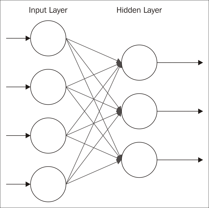
The number of input nodes for the visible layer is dependent on the problem being solved. For example, if we are looking at an image with 256 pixels, then we will need 256 input nodes. For an image, this is the number of rows times the number of columns for the image.
The Hidden Layer should contain fewer neurons than the Input Layer. Using close to the same number of neurons will sometimes result in the construction of an identity function. Too many neurons may result in overfitting. This means that datasets with a large number of inputs will require multiple layers. Smaller input sizes result in the need for fewer layers.
Stochastic, that is, random, values are assigned to each node's weights. The value for a node is multiplied by its weight and then added to a bias. This value, combined with the combined input from the other input nodes, is then fed into the activation function, where an output value is generated.
The RBM technique goes through a reconstruction phase. This is where the activations are fed back to the first layer and multiplied by the same weights used for the input. The sum of these values from each node of the second layer, plus another bias, represents an approximation of the original input. The idea is to train the model to minimize the difference between the original input values and the feedback values.
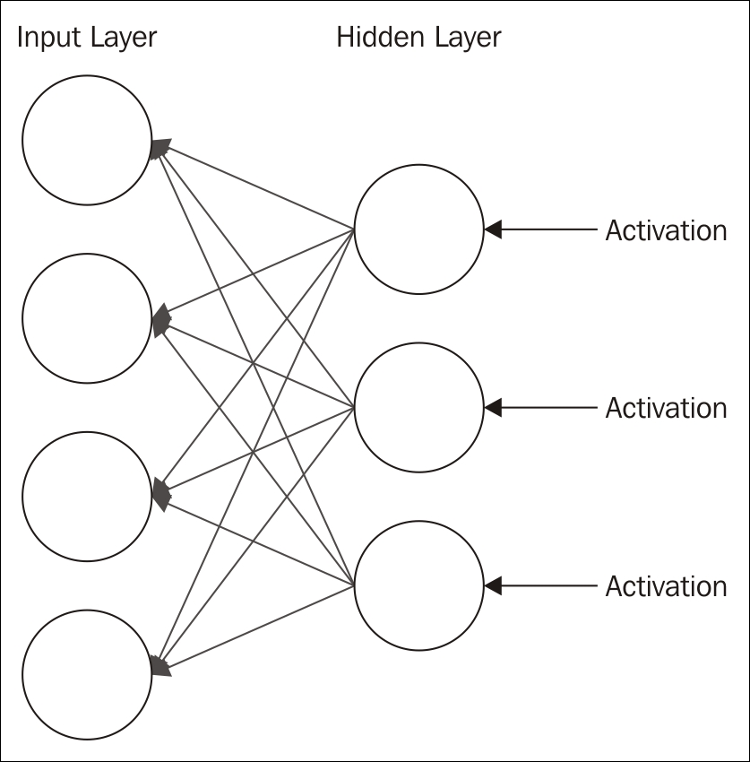
The difference in values is treated as an error. The process is repeated until an error minimum is reached. You can think of the reconstruction as guesses about the original input. These guesses are essentially a probability distribution of the original input. This is called generative learning, in contrast to discriminative learning, which occurs with classification techniques.
In a multi-layer model, each layer can be used to essentially identify a feature. In subsequent layers, a combination of features may be identified or generated. In this way, a seemingly random set of pixel values may be analyzed to identify the veins of a leaf, a leaf, a trunk, and then a tree.
The output of an RBM is a value that essentially represents a percentage. If it is not zero, then the machine has learned something about the input.
We will examine two different RBM configurations. The first one is minimal and we will see it again in Deep autoencoders. The second uses several additional methods and provides more insights into the various ways it can be configured.
The following statement creates a new layer using the RBM.Builder class. The input is computed based on the number of rows and columns of an image. The output is large, containing 1000 neurons. The loss function is RMSE_XENT. This loss function works better for some classification problems:
.layer(0, new RBM.Builder()
.nIn(numRows * numColumns).nOut(1000)
.lossFunction(LossFunctions.LossFunction.RMSE_XENT)
.build())
Next is a more complex RBM. We will not detail each of these methods here but will see them used in later examples:
.layer(new RBM.Builder()
.l2(1e-1).l1(1e-3)
.nIn(numRows * numColumns
.nOut(outputNum)
.activation("relu")
.weightInit(WeightInit.RELU)
.lossFunction(LossFunctions.LossFunction
.RECONSTRUCTION_CROSSENTROPY).k(3)
.hiddenUnit(HiddenUnit.RECTIFIED)
.visibleUnit(VisibleUnit.GAUSSIAN)
.updater(Updater.ADAGRAD)
.gradientNormalization(
GradientNormalization.ClipL2PerLayer)
.build())
A single-layer RBM is not always useful. A multi-layer autoencoder is often required. We will look at this option in the next section.
Reconstruction in an RBM
The RBM technique goes through a reconstruction phase. This is where the activations are fed back to the first layer and multiplied by the same weights used for the input. The sum of these values from each node of the second layer, plus another bias, represents an approximation of the original input. The idea is to train the model to minimize the difference between the original input values and the feedback values.
The difference in values is treated as an error. The process is repeated until an error minimum is reached. You can think of the reconstruction as guesses about the original input. These guesses are essentially a probability distribution of the original input. This is called generative learning, in contrast to discriminative learning, which occurs with classification techniques.
In a multi-layer model, each layer can be used to essentially identify a feature. In subsequent layers, a combination of features may be identified or generated. In this way, a seemingly random set of pixel values may be analyzed to identify the veins of a leaf, a leaf, a trunk, and then a tree.
The output of an RBM is a value that essentially represents a percentage. If it is not zero, then the machine has learned something about the input.
We will examine two different RBM configurations. The first one is minimal and we will see it again in Deep autoencoders. The second uses several additional methods and provides more insights into the various ways it can be configured.
The following statement creates a new layer using the RBM.Builder class. The input is computed based on the number of rows and columns of an image. The output is large, containing 1000 neurons. The loss function is RMSE_XENT. This loss function works better for some classification problems:
.layer(0, new RBM.Builder()
.nIn(numRows * numColumns).nOut(1000)
.lossFunction(LossFunctions.LossFunction.RMSE_XENT)
.build())
Next is a more complex RBM. We will not detail each of these methods here but will see them used in later examples:
.layer(new RBM.Builder()
.l2(1e-1).l1(1e-3)
.nIn(numRows * numColumns
.nOut(outputNum)
.activation("relu")
.weightInit(WeightInit.RELU)
.lossFunction(LossFunctions.LossFunction
.RECONSTRUCTION_CROSSENTROPY).k(3)
.hiddenUnit(HiddenUnit.RECTIFIED)
.visibleUnit(VisibleUnit.GAUSSIAN)
.updater(Updater.ADAGRAD)
.gradientNormalization(
GradientNormalization.ClipL2PerLayer)
.build())
A single-layer RBM is not always useful. A multi-layer autoencoder is often required. We will look at this option in the next section.
Configuring an RBM
We will examine two different RBM configurations. The first one is minimal and we will see it again in Deep autoencoders. The second uses several additional methods and provides more insights into the various ways it can be configured.
The following statement creates a new layer using the RBM.Builder class. The input is computed based on the number of rows and columns of an image. The output is large, containing 1000 neurons. The loss function is RMSE_XENT. This loss function works better for some classification problems:
.layer(0, new RBM.Builder()
.nIn(numRows * numColumns).nOut(1000)
.lossFunction(LossFunctions.LossFunction.RMSE_XENT)
.build())
Next is a more complex RBM. We will not detail each of these methods here but will see them used in later examples:
.layer(new RBM.Builder()
.l2(1e-1).l1(1e-3)
.nIn(numRows * numColumns
.nOut(outputNum)
.activation("relu")
.weightInit(WeightInit.RELU)
.lossFunction(LossFunctions.LossFunction
.RECONSTRUCTION_CROSSENTROPY).k(3)
.hiddenUnit(HiddenUnit.RECTIFIED)
.visibleUnit(VisibleUnit.GAUSSIAN)
.updater(Updater.ADAGRAD)
.gradientNormalization(
GradientNormalization.ClipL2PerLayer)
.build())
A single-layer RBM is not always useful. A multi-layer autoencoder is often required. We will look at this option in the next section.
An autoencoder is used for feature selection and extraction. It consists of two symmetrical DBNs. The first half of the network is composed of several layers, which performs encoding. The second part of the network performs decoding. Each layer of the autoencoder is an RBM. This is illustrated in the following figure:
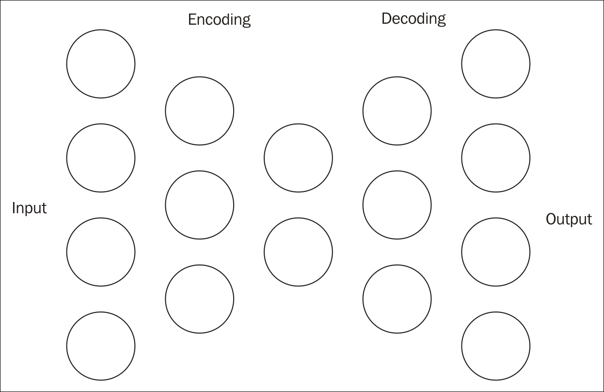
The purpose of the encoding sequence is to compress the original input into a smaller vector space. The middle layer of the previous figure is this compressed layer. These intermediate vectors can be thought of as possible features of the dataset. The encoding is also referred to as the pre-training half. It is the output of the intermediate RBM layer and does not perform classification.
The encoder's first layer will use more inputs than used by the dataset. This has the effect of expanding the features of the dataset. A sigmoid-belief unit is a form of non-linear transformation used with each layer. This unit is not able to accurately represent information as real values. However, using more inputs, it is able to do a better job.
The second half of the network performs decoding, effectively reconstructing the input. This is a forward-feed network, using the same weights as the corresponding layers in the encoding half. However, the weights are transposed and are not initialized randomly. The training rate needs to be set lower for the second half.
An autoencoder is useful for data compression and searching. The output of the first half of the model is compressed, thus making it useful for storage and transmission usage. Later, it can be decompressed, as we will demonstrate in Chapter 10, Visual and Audio Analysis. This is sometimes referred to as semantic hashing.
If a series of inputs, such as images or sounds, have been compressed and stored, then new input can be compressed and matched with the stored values to find the best fit. An autoencoder can also be used for other information retrieval tasks.
This example is adapted from http://deeplearning4j.org/deepautoencoder. We start with a try-catch block to handle errors that may crop up and with a few variable declarations. This example uses the Mnist (http://yann.lecun.com/exdb/mnist/) dataset, which is a set of images containing hand-written numbers. Each image consists of 28 by 28 pixels. An iterator is declared to access the data:
try {
final int numberOfRows = 28;
final int numberOfColumns = 28;
int seed = 123;
int numberOfIterations = 1;
iterator = new MnistDataSetIterator(
1000, MnistDataFetcher.NUM_EXAMPLES, true);
...
} catch (IOException ex) {
// Handle exceptions
}
The configuration of the network is created using the NeuralNetConfiguration.Builder() class. Ten layers are created where the input layer consists of 1000 neurons. This is larger than the 28 by 28 pixel input and is used to compensate for the sigmoid-belief units used in each layer.
Each of the subsequent layers gets smaller until layer four is reached. This layer represents the last step of the encoding process. With layer five, the decoding process starts and the subsequent layers get bigger. The last layer uses 1000 neurons.
Each layer of the model uses an RBM instance except the last layer, which is constructed using the OutputLayer.Builder class. The configuration code follows:
MultiLayerConfiguration conf = new NeuralNetConfiguration.Builder()
.seed(seed)
.iterations(numberOfIterations)
.optimizationAlgo(
OptimizationAlgorithm.LINE_GRADIENT_DESCENT)
.list()
.layer(0, new RBM.Builder()
.nIn(numberOfRows * numberOfColumns).nOut(1000)
.lossFunction(LossFunctions.LossFunction.RMSE_XENT)
.build())
.layer(1, new RBM.Builder().nIn(1000).nOut(500)
.lossFunction(LossFunctions.LossFunction.RMSE_XENT)
.build())
.layer(2, new RBM.Builder().nIn(500).nOut(250)
.lossFunction(LossFunctions.LossFunction.RMSE_XENT)
.build())
.layer(3, new RBM.Builder().nIn(250).nOut(100)
.lossFunction(LossFunctions.LossFunction.RMSE_XENT)
.build())
.layer(4, new RBM.Builder().nIn(100).nOut(30)
.lossFunction(LossFunctions.LossFunction.RMSE_XENT)
.build()) //encoding stops
.layer(5, new RBM.Builder().nIn(30).nOut(100)
.lossFunction(LossFunctions.LossFunction.RMSE_XENT)
.build()) //decoding starts
.layer(6, new RBM.Builder().nIn(100).nOut(250)
.lossFunction(LossFunctions.LossFunction.RMSE_XENT)
.build())
.layer(7, new RBM.Builder().nIn(250).nOut(500)
.lossFunction(LossFunctions.LossFunction.RMSE_XENT)
.build())
.layer(8, new RBM.Builder().nIn(500).nOut(1000)
.lossFunction(LossFunctions.LossFunction.RMSE_XENT)
.build())
.layer(9, new OutputLayer.Builder(
LossFunctions.LossFunction.RMSE_XENT).nIn(1000)
.nOut(numberOfRows * numberOfColumns).build())
.pretrain(true).backprop(true)
.build();
The model is then created and initialized, and score iteration listeners are set up:
model = new MultiLayerNetwork(conf);
model.init();
model.setListeners(Collections.singletonList(
(IterationListener) new ScoreIterationListener()));
The model is trained using the fit method:
while (iterator.hasNext()) {
DataSet dataSet = iterator.next();
model.fit(new DataSet(dataSet.getFeatureMatrix(),
dataSet.getFeatureMatrix()));
}
It is useful to save the model so that it can be used for later analysis. This is accomplished using the ModelSerializer class's writeModel method. It takes the model instance and modelFile instance, along with a boolean parameter specifying whether the model's updater should be saved. An updater is a learning algorithm used for adjusting certain model parameters:
modelFile = new File("savedModel");
ModelSerializer.writeModel(model, modelFile, true);
The model can be retrieved using the following code:
modelFile = new File("savedModel");
MultiLayerNetwork model = ModelSerializer.restoreMultiLayerNetwork(modelFile);
There are specialized versions of autoencoders. When an autoencoder uses more hidden layers than inputs, it may learn the identity function, which is a function that always returns the same value used as input to the function. To avoid this problem, an extension to the autoencoder, denoising autoencoder, is used; it randomly modifies the input introducing noise. The amount of noise introduced varies depending on the input dataset. A Stacked Denoising Autoencoder (SdA) is a series of denoising autoencoders strung together.
Building an autoencoder in DL4J
This example is adapted from http://deeplearning4j.org/deepautoencoder. We start with a try-catch block to handle errors that may crop up and with a few variable declarations. This example uses the Mnist (http://yann.lecun.com/exdb/mnist/) dataset, which is a set of images containing hand-written numbers. Each image consists of 28 by 28 pixels. An iterator is declared to access the data:
try {
final int numberOfRows = 28;
final int numberOfColumns = 28;
int seed = 123;
int numberOfIterations = 1;
iterator = new MnistDataSetIterator(
1000, MnistDataFetcher.NUM_EXAMPLES, true);
...
} catch (IOException ex) {
// Handle exceptions
}
The configuration of the network is created using the NeuralNetConfiguration.Builder() class. Ten layers are created where the input layer consists of 1000 neurons. This is larger than the 28 by 28 pixel input and is used to compensate for the sigmoid-belief units used in each layer.
Each of the subsequent layers gets smaller until layer four is reached. This layer represents the last step of the encoding process. With layer five, the decoding process starts and the subsequent layers get bigger. The last layer uses 1000 neurons.
Each layer of the model uses an RBM instance except the last layer, which is constructed using the OutputLayer.Builder class. The configuration code follows:
MultiLayerConfiguration conf = new NeuralNetConfiguration.Builder()
.seed(seed)
.iterations(numberOfIterations)
.optimizationAlgo(
OptimizationAlgorithm.LINE_GRADIENT_DESCENT)
.list()
.layer(0, new RBM.Builder()
.nIn(numberOfRows * numberOfColumns).nOut(1000)
.lossFunction(LossFunctions.LossFunction.RMSE_XENT)
.build())
.layer(1, new RBM.Builder().nIn(1000).nOut(500)
.lossFunction(LossFunctions.LossFunction.RMSE_XENT)
.build())
.layer(2, new RBM.Builder().nIn(500).nOut(250)
.lossFunction(LossFunctions.LossFunction.RMSE_XENT)
.build())
.layer(3, new RBM.Builder().nIn(250).nOut(100)
.lossFunction(LossFunctions.LossFunction.RMSE_XENT)
.build())
.layer(4, new RBM.Builder().nIn(100).nOut(30)
.lossFunction(LossFunctions.LossFunction.RMSE_XENT)
.build()) //encoding stops
.layer(5, new RBM.Builder().nIn(30).nOut(100)
.lossFunction(LossFunctions.LossFunction.RMSE_XENT)
.build()) //decoding starts
.layer(6, new RBM.Builder().nIn(100).nOut(250)
.lossFunction(LossFunctions.LossFunction.RMSE_XENT)
.build())
.layer(7, new RBM.Builder().nIn(250).nOut(500)
.lossFunction(LossFunctions.LossFunction.RMSE_XENT)
.build())
.layer(8, new RBM.Builder().nIn(500).nOut(1000)
.lossFunction(LossFunctions.LossFunction.RMSE_XENT)
.build())
.layer(9, new OutputLayer.Builder(
LossFunctions.LossFunction.RMSE_XENT).nIn(1000)
.nOut(numberOfRows * numberOfColumns).build())
.pretrain(true).backprop(true)
.build();
The model is then created and initialized, and score iteration listeners are set up:
model = new MultiLayerNetwork(conf);
model.init();
model.setListeners(Collections.singletonList(
(IterationListener) new ScoreIterationListener()));
The model is trained using the fit method:
while (iterator.hasNext()) {
DataSet dataSet = iterator.next();
model.fit(new DataSet(dataSet.getFeatureMatrix(),
dataSet.getFeatureMatrix()));
}
It is useful to save the model so that it can be used for later analysis. This is accomplished using the ModelSerializer class's writeModel method. It takes the model instance and modelFile instance, along with a boolean parameter specifying whether the model's updater should be saved. An updater is a learning algorithm used for adjusting certain model parameters:
modelFile = new File("savedModel");
ModelSerializer.writeModel(model, modelFile, true);
The model can be retrieved using the following code:
modelFile = new File("savedModel");
MultiLayerNetwork model = ModelSerializer.restoreMultiLayerNetwork(modelFile);
There are specialized versions of autoencoders. When an autoencoder uses more hidden layers than inputs, it may learn the identity function, which is a function that always returns the same value used as input to the function. To avoid this problem, an extension to the autoencoder, denoising autoencoder, is used; it randomly modifies the input introducing noise. The amount of noise introduced varies depending on the input dataset. A Stacked Denoising Autoencoder (SdA) is a series of denoising autoencoders strung together.
Configuring the network
The configuration of the network is created using the NeuralNetConfiguration.Builder() class. Ten layers are created where the input layer consists of 1000 neurons. This is larger than the 28 by 28 pixel input and is used to compensate for the sigmoid-belief units used in each layer.
Each of the subsequent layers gets smaller until layer four is reached. This layer represents the last step of the encoding process. With layer five, the decoding process starts and the subsequent layers get bigger. The last layer uses 1000 neurons.
Each layer of the model uses an RBM instance except the last layer, which is constructed using the OutputLayer.Builder class. The configuration code follows:
MultiLayerConfiguration conf = new NeuralNetConfiguration.Builder()
.seed(seed)
.iterations(numberOfIterations)
.optimizationAlgo(
OptimizationAlgorithm.LINE_GRADIENT_DESCENT)
.list()
.layer(0, new RBM.Builder()
.nIn(numberOfRows * numberOfColumns).nOut(1000)
.lossFunction(LossFunctions.LossFunction.RMSE_XENT)
.build())
.layer(1, new RBM.Builder().nIn(1000).nOut(500)
.lossFunction(LossFunctions.LossFunction.RMSE_XENT)
.build())
.layer(2, new RBM.Builder().nIn(500).nOut(250)
.lossFunction(LossFunctions.LossFunction.RMSE_XENT)
.build())
.layer(3, new RBM.Builder().nIn(250).nOut(100)
.lossFunction(LossFunctions.LossFunction.RMSE_XENT)
.build())
.layer(4, new RBM.Builder().nIn(100).nOut(30)
.lossFunction(LossFunctions.LossFunction.RMSE_XENT)
.build()) //encoding stops
.layer(5, new RBM.Builder().nIn(30).nOut(100)
.lossFunction(LossFunctions.LossFunction.RMSE_XENT)
.build()) //decoding starts
.layer(6, new RBM.Builder().nIn(100).nOut(250)
.lossFunction(LossFunctions.LossFunction.RMSE_XENT)
.build())
.layer(7, new RBM.Builder().nIn(250).nOut(500)
.lossFunction(LossFunctions.LossFunction.RMSE_XENT)
.build())
.layer(8, new RBM.Builder().nIn(500).nOut(1000)
.lossFunction(LossFunctions.LossFunction.RMSE_XENT)
.build())
.layer(9, new OutputLayer.Builder(
LossFunctions.LossFunction.RMSE_XENT).nIn(1000)
.nOut(numberOfRows * numberOfColumns).build())
.pretrain(true).backprop(true)
.build();
The model is then created and initialized, and score iteration listeners are set up:
model = new MultiLayerNetwork(conf);
model.init();
model.setListeners(Collections.singletonList(
(IterationListener) new ScoreIterationListener()));
The model is trained using the fit method:
while (iterator.hasNext()) {
DataSet dataSet = iterator.next();
model.fit(new DataSet(dataSet.getFeatureMatrix(),
dataSet.getFeatureMatrix()));
}
It is useful to save the model so that it can be used for later analysis. This is accomplished using the ModelSerializer class's writeModel method. It takes the model instance and modelFile instance, along with a boolean parameter specifying whether the model's updater should be saved. An updater is a learning algorithm used for adjusting certain model parameters:
modelFile = new File("savedModel");
ModelSerializer.writeModel(model, modelFile, true);
The model can be retrieved using the following code:
modelFile = new File("savedModel");
MultiLayerNetwork model = ModelSerializer.restoreMultiLayerNetwork(modelFile);
There are specialized versions of autoencoders. When an autoencoder uses more hidden layers than inputs, it may learn the identity function, which is a function that always returns the same value used as input to the function. To avoid this problem, an extension to the autoencoder, denoising autoencoder, is used; it randomly modifies the input introducing noise. The amount of noise introduced varies depending on the input dataset. A Stacked Denoising Autoencoder (SdA) is a series of denoising autoencoders strung together.
Building and training the network
The model is then created and initialized, and score iteration listeners are set up:
model = new MultiLayerNetwork(conf);
model.init();
model.setListeners(Collections.singletonList(
(IterationListener) new ScoreIterationListener()));
The model is trained using the fit method:
while (iterator.hasNext()) {
DataSet dataSet = iterator.next();
model.fit(new DataSet(dataSet.getFeatureMatrix(),
dataSet.getFeatureMatrix()));
}
It is useful to save the model so that it can be used for later analysis. This is accomplished using the ModelSerializer class's writeModel method. It takes the model instance and modelFile instance, along with a boolean parameter specifying whether the model's updater should be saved. An updater is a learning algorithm used for adjusting certain model parameters:
modelFile = new File("savedModel");
ModelSerializer.writeModel(model, modelFile, true);
The model can be retrieved using the following code:
modelFile = new File("savedModel");
MultiLayerNetwork model = ModelSerializer.restoreMultiLayerNetwork(modelFile);
There are specialized versions of autoencoders. When an autoencoder uses more hidden layers than inputs, it may learn the identity function, which is a function that always returns the same value used as input to the function. To avoid this problem, an extension to the autoencoder, denoising autoencoder, is used; it randomly modifies the input introducing noise. The amount of noise introduced varies depending on the input dataset. A Stacked Denoising Autoencoder (SdA) is a series of denoising autoencoders strung together.
Saving and retrieving a network
It is useful to save the model so that it can be used for later analysis. This is accomplished using the ModelSerializer class's writeModel method. It takes the model instance and modelFile instance, along with a boolean parameter specifying whether the model's updater should be saved. An updater is a learning algorithm used for adjusting certain model parameters:
modelFile = new File("savedModel");
ModelSerializer.writeModel(model, modelFile, true);
The model can be retrieved using the following code:
modelFile = new File("savedModel");
MultiLayerNetwork model = ModelSerializer.restoreMultiLayerNetwork(modelFile);
There are specialized versions of autoencoders. When an autoencoder uses more hidden layers than inputs, it may learn the identity function, which is a function that always returns the same value used as input to the function. To avoid this problem, an extension to the autoencoder, denoising autoencoder, is used; it randomly modifies the input introducing noise. The amount of noise introduced varies depending on the input dataset. A Stacked Denoising Autoencoder (SdA) is a series of denoising autoencoders strung together.
Specialized autoencoders
There are specialized versions of autoencoders. When an autoencoder uses more hidden layers than inputs, it may learn the identity function, which is a function that always returns the same value used as input to the function. To avoid this problem, an extension to the autoencoder, denoising autoencoder, is used; it randomly modifies the input introducing noise. The amount of noise introduced varies depending on the input dataset. A Stacked Denoising Autoencoder (SdA) is a series of denoising autoencoders strung together.
CNNs are feed-forward networks modeled after the visual cortex found in animals. The visual cortex is arranged with overlapping neurons, and so in this type of network, the neurons are also arranged in overlapping sections, known as receptive fields. Due to their design model, they function with minimal preprocessing or prior knowledge, and this lack of human intervention makes them especially useful.
This type of network is used frequently in image and video recognition applications. They can be used for classification, clustering, and object recognition. CNNs can also be applied to text analysis by implementing Optical Character Recognition (OCR). CNNs have been a driving force in the machine learning movement in part due to their wide applicability in practical situations.
We are going to demonstrate a CNN using DL4J. The process will closely mirror the process we used in the Building an autoencoder in DL4J section. We will again use the Mnist dataset. This dataset contains image data, so it is well-suited to a convolutional network.
First, we need to create a new DataSetIterator to process the data. The parameters for the MnistDataSetIterator constructor are the batch size, 1000 in this case, and the total number of samples to process. We then get our next dataset, shuffle the data to randomize, and split our data to be tested and trained. As we discussed earlier in the chapter, we typically use 65% of the data to train the data and the remaining 35% is used for testing:
DataSetIterator iter = new MnistDataSetIterator(1000, MnistDataFetcher.NUM_EXAMPLES); DataSet dataset = iter.next(); dataset.shuffle(); SplitTestAndTrain testAndTrain = dataset.splitTestAndTrain(0.65); DataSet trainingData = testAndTrain.getTrain(); DataSet testData = testAndTrain.getTest();
We then normalize both sets of data:
DataNormalization normalizer = new NormalizerStandardize(); normalizer.fit(trainingData); normalizer.transform(trainingData); normalizer.transform(testData);
Next, we can build our network. As shown earlier, we will again use a MultiLayerConfiguration instance with a series of NeuralNetConfiguration.Builder methods. We will discuss the individual methods after the following code sequence. Notice that the last layer again uses the softmax activation function for regression analysis:
MultiLayerConfiguration.Builder builder = new
NeuralNetConfiguration.Builder()
.seed(123)
.iterations(1)
.regularization(true).l2(0.0005)
.weightInit(WeightInit.XAVIER)
.optimizationAlgo(OptimizationAlgorithm
.STOCHASTIC_GRADIENT_DESCENT)
.updater(Updater.NESTEROVS).momentum(0.9)
.list()
.layer(0, new ConvolutionLayer.Builder(5, 5)
.nIn(6)
.stride(1, 1)
.nOut(20)
.activation("identity")
.build())
.layer(1, new SubsamplingLayer.Builder(
SubsamplingLayer.PoolingType.MAX)
.kernelSize(2, 2)
.stride(2, 2)
.build())
.layer(2, new ConvolutionLayer.Builder(5, 5)
.stride(1, 1)
.nOut(50)
.activation("identity")
.build())
.layer(3, new SubsamplingLayer.Builder(
SubsamplingLayer.PoolingType.MAX)
.kernelSize(2, 2)
.stride(2, 2)
.build())
.layer(4, new DenseLayer.Builder().activation("relu")
.nOut(500).build())
.layer(5, new OutputLayer.Builder(
LossFunctions.LossFunction.NEGATIVELOGLIKELIHOOD)
.nOut(10)
.activation("softmax")
.build())
.backprop(true).pretrain(false);
The first layer, layer 0, which is duplicated next for your convenience, uses the ConvolutionLayer.Builder method. The input to a convolution layer is the product of the image height, width, and number of channels. In a standard RGB image, there are three channels. The nIn method takes the number of channels. The nOut method specifies that 20 outputs are expected:
.layer(0, new ConvolutionLayer.Builder(5, 5)
.nIn(6)
.stride(1, 1)
.nOut(20)
.activation("identity")
.build())
Layers 1 and 3 are both subsampling layers. These layers follow convolution layers and do no real convolution themselves. They return a single value, the maximum value for that input region:
.layer(1, new SubsamplingLayer.Builder(
SubsamplingLayer.PoolingType.MAX)
.kernelSize(2, 2)
.stride(2, 2)
.build())
...
.layer(3, new SubsamplingLayer.Builder(
SubsamplingLayer.PoolingType.MAX)
.kernelSize(2, 2)
.stride(2, 2)
.build())
Layer 2 is also a convolution layer like layer 0. Notice that we do not specify the number of channels in this layer:
.layer(2, new ConvolutionLayer.Builder(5, 5)
.nOut(50)
.activation("identity")
.build())
The fourth layer uses the DenseLayer.Builder class, as in our earlier example. As mentioned previously, the DenseLayer class is a feed-forward and fully connected layer:
.layer(4, new DenseLayer.Builder().activation("relu")
.nOut(500).build())
The layer 5 is an OutputLayer instance and uses softmax automation:
.layer(5, new OutputLayer.Builder(
LossFunctions.LossFunction.NEGATIVELOGLIKELIHOOD)
.nOut(10)
.activation("softmax")
.build())
.backprop(true).pretrain(false);
Finally, we create a new instance of the ConvolutionalLayerSetup class. We pass the builder object and the dimensions of our image (28 x 28). We also pass the number of channels, in this case, 1:
new ConvolutionLayerSetup(builder, 28, 28, 1);
We can now configure and fit our model. We once again use the MultiLayerConfiguration and MultiLayerNetwork classes to build our network. We set up listeners and then iterate through our data. For each DataSet, we execute the fit method:
MultiLayerConfiguration conf = builder.build();
MultiLayerNetwork model = new MultiLayerNetwork(conf);
model.init();
model.setListeners(Collections.singletonList((IterationListener)
new ScoreIterationListener(1/5)));
while (iter.hasNext()) {
DataSet next = iter.next();
model.fit(new DataSet(next.getFeatureMatrix(), next.getLabels()));
}
We are now ready to evaluate our model.
To evaluate our model, we use the Evaluation class. We get the output from our model and send it, along with the labels for our dataset, to the eval method. We then execute the stats method to get the statistical information on our network:
Evaluation evaluation = new Evaluation(4); INDArray output = model.output(testData.getFeatureMatrix()); evaluation.eval(testData.getLabels(), output); out.println(evaluation.stats());
The following is a sample output from the execution of this code, for we are only showing the results of the stats method. The first part reports on how examples are classified and the second part displays various statistics:
Examples labeled as 0 classified by model as 0: 19 times Examples labeled as 1 classified by model as 1: 41 times Examples labeled as 2 classified by model as 1: 4 times Examples labeled as 2 classified by model as 2: 30 times Examples labeled as 2 classified by model as 3: 1 times Examples labeled as 3 classified by model as 2: 1 times Examples labeled as 3 classified by model as 3: 28 times ==========================Scores===================================Accuracy: 0.3371 Precision: 0.8481 Recall: 0.8475 F1 Score: 0.8478 ===================================================================
As in our previous model, the evaluation demonstrates decent accuracy and success with our network.
Building the model
First, we need to create a new DataSetIterator to process the data. The parameters for the MnistDataSetIterator constructor are the batch size, 1000 in this case, and the total number of samples to process. We then get our next dataset, shuffle the data to randomize, and split our data to be tested and trained. As we discussed earlier in the chapter, we typically use 65% of the data to train the data and the remaining 35% is used for testing:
DataSetIterator iter = new MnistDataSetIterator(1000, MnistDataFetcher.NUM_EXAMPLES); DataSet dataset = iter.next(); dataset.shuffle(); SplitTestAndTrain testAndTrain = dataset.splitTestAndTrain(0.65); DataSet trainingData = testAndTrain.getTrain(); DataSet testData = testAndTrain.getTest();
We then normalize both sets of data:
DataNormalization normalizer = new NormalizerStandardize(); normalizer.fit(trainingData); normalizer.transform(trainingData); normalizer.transform(testData);
Next, we can build our network. As shown earlier, we will again use a MultiLayerConfiguration instance with a series of NeuralNetConfiguration.Builder methods. We will discuss the individual methods after the following code sequence. Notice that the last layer again uses the softmax activation function for regression analysis:
MultiLayerConfiguration.Builder builder = new
NeuralNetConfiguration.Builder()
.seed(123)
.iterations(1)
.regularization(true).l2(0.0005)
.weightInit(WeightInit.XAVIER)
.optimizationAlgo(OptimizationAlgorithm
.STOCHASTIC_GRADIENT_DESCENT)
.updater(Updater.NESTEROVS).momentum(0.9)
.list()
.layer(0, new ConvolutionLayer.Builder(5, 5)
.nIn(6)
.stride(1, 1)
.nOut(20)
.activation("identity")
.build())
.layer(1, new SubsamplingLayer.Builder(
SubsamplingLayer.PoolingType.MAX)
.kernelSize(2, 2)
.stride(2, 2)
.build())
.layer(2, new ConvolutionLayer.Builder(5, 5)
.stride(1, 1)
.nOut(50)
.activation("identity")
.build())
.layer(3, new SubsamplingLayer.Builder(
SubsamplingLayer.PoolingType.MAX)
.kernelSize(2, 2)
.stride(2, 2)
.build())
.layer(4, new DenseLayer.Builder().activation("relu")
.nOut(500).build())
.layer(5, new OutputLayer.Builder(
LossFunctions.LossFunction.NEGATIVELOGLIKELIHOOD)
.nOut(10)
.activation("softmax")
.build())
.backprop(true).pretrain(false);
The first layer, layer 0, which is duplicated next for your convenience, uses the ConvolutionLayer.Builder method. The input to a convolution layer is the product of the image height, width, and number of channels. In a standard RGB image, there are three channels. The nIn method takes the number of channels. The nOut method specifies that 20 outputs are expected:
.layer(0, new ConvolutionLayer.Builder(5, 5)
.nIn(6)
.stride(1, 1)
.nOut(20)
.activation("identity")
.build())
Layers 1 and 3 are both subsampling layers. These layers follow convolution layers and do no real convolution themselves. They return a single value, the maximum value for that input region:
.layer(1, new SubsamplingLayer.Builder(
SubsamplingLayer.PoolingType.MAX)
.kernelSize(2, 2)
.stride(2, 2)
.build())
...
.layer(3, new SubsamplingLayer.Builder(
SubsamplingLayer.PoolingType.MAX)
.kernelSize(2, 2)
.stride(2, 2)
.build())
Layer 2 is also a convolution layer like layer 0. Notice that we do not specify the number of channels in this layer:
.layer(2, new ConvolutionLayer.Builder(5, 5)
.nOut(50)
.activation("identity")
.build())
The fourth layer uses the DenseLayer.Builder class, as in our earlier example. As mentioned previously, the DenseLayer class is a feed-forward and fully connected layer:
.layer(4, new DenseLayer.Builder().activation("relu")
.nOut(500).build())
The layer 5 is an OutputLayer instance and uses softmax automation:
.layer(5, new OutputLayer.Builder(
LossFunctions.LossFunction.NEGATIVELOGLIKELIHOOD)
.nOut(10)
.activation("softmax")
.build())
.backprop(true).pretrain(false);
Finally, we create a new instance of the ConvolutionalLayerSetup class. We pass the builder object and the dimensions of our image (28 x 28). We also pass the number of channels, in this case, 1:
new ConvolutionLayerSetup(builder, 28, 28, 1);
We can now configure and fit our model. We once again use the MultiLayerConfiguration and MultiLayerNetwork classes to build our network. We set up listeners and then iterate through our data. For each DataSet, we execute the fit method:
MultiLayerConfiguration conf = builder.build();
MultiLayerNetwork model = new MultiLayerNetwork(conf);
model.init();
model.setListeners(Collections.singletonList((IterationListener)
new ScoreIterationListener(1/5)));
while (iter.hasNext()) {
DataSet next = iter.next();
model.fit(new DataSet(next.getFeatureMatrix(), next.getLabels()));
}
We are now ready to evaluate our model.
To evaluate our model, we use the Evaluation class. We get the output from our model and send it, along with the labels for our dataset, to the eval method. We then execute the stats method to get the statistical information on our network:
Evaluation evaluation = new Evaluation(4); INDArray output = model.output(testData.getFeatureMatrix()); evaluation.eval(testData.getLabels(), output); out.println(evaluation.stats());
The following is a sample output from the execution of this code, for we are only showing the results of the stats method. The first part reports on how examples are classified and the second part displays various statistics:
Examples labeled as 0 classified by model as 0: 19 times Examples labeled as 1 classified by model as 1: 41 times Examples labeled as 2 classified by model as 1: 4 times Examples labeled as 2 classified by model as 2: 30 times Examples labeled as 2 classified by model as 3: 1 times Examples labeled as 3 classified by model as 2: 1 times Examples labeled as 3 classified by model as 3: 28 times ==========================Scores===================================Accuracy: 0.3371 Precision: 0.8481 Recall: 0.8475 F1 Score: 0.8478 ===================================================================
As in our previous model, the evaluation demonstrates decent accuracy and success with our network.
Evaluating the model
To evaluate our model, we use the Evaluation class. We get the output from our model and send it, along with the labels for our dataset, to the eval method. We then execute the stats method to get the statistical information on our network:
Evaluation evaluation = new Evaluation(4); INDArray output = model.output(testData.getFeatureMatrix()); evaluation.eval(testData.getLabels(), output); out.println(evaluation.stats());
The following is a sample output from the execution of this code, for we are only showing the results of the stats method. The first part reports on how examples are classified and the second part displays various statistics:
Examples labeled as 0 classified by model as 0: 19 times Examples labeled as 1 classified by model as 1: 41 times Examples labeled as 2 classified by model as 1: 4 times Examples labeled as 2 classified by model as 2: 30 times Examples labeled as 2 classified by model as 3: 1 times Examples labeled as 3 classified by model as 2: 1 times Examples labeled as 3 classified by model as 3: 28 times ==========================Scores===================================Accuracy: 0.3371 Precision: 0.8481 Recall: 0.8475 F1 Score: 0.8478 ===================================================================
As in our previous model, the evaluation demonstrates decent accuracy and success with our network.
RNN differ from feed-forward networks in that their input includes the input from the previous iteration or step. They still process the current input but use a feedback loop to take into consideration the inputs to the prior step, also called the recent past, for context. This step effectively gives the network memory. One popular type of recurrent network involves Long Short-Term Memory (LSTM). This type of memory improves the processing power of the network.
RNNs are designed to process sequential data and are especially useful for analysis and prediction with text data. Given a sequence of words, an RNN can predict the probability of each word being the next in the sequence. This also allows for text generation by the network. RNNs are versatile and also process image data well, especially image labeling applications. The flexibility in design and purpose and ease in training make RNNs popular choices for many data science applications. DL4J also provides support for LSTM networks and other RNNs.
In this chapter, we examined deep learning techniques for neural networks. All API support in this chapter was provided by Deeplearning4j. We began by demonstrating how to acquire and prepare data for use with deep learning networks. We discussed how to configure and build a model. This was followed by an explanation of how to train and test a model by splitting the dataset into training and testing segments.
Our discussion continued with an examination of deep learning and regression analysis. We showed how to prepare the data and class, build the model, and evaluate the model. We used sample data and displayed output statistics to demonstrate the relative effectiveness of our model.
RBM and DBNs were then examined. DBNs are comprised of RBMs stacked together and are especially useful for classification and clustering applications. Deep autoencoders are also built using RBMs, with two symmetrical DBNs. The autoencoders are especially useful for feature selection and extraction.
Finally, we demonstrated a convolutional network. This network is modeled after the visual cortex and allows the network to use regions of information for classification. As in previous examples, we built, trained, and then evaluated the model for effectiveness. We then concluded the chapter with a brief introduction to recurrent neural networks.
We will expand upon these topics as we move into next chapter and examine text analysis techniques.