

The concurrent execution of a program can result in significant performance improvements. In this chapter, we will address the various techniques that can be used in data science applications. These can range from low-level mathematical calculations to higher-level API-specific options.
Always keep in mind that performance enhancement starts with ensuring that the correct set of application functionality is implemented. If the application does not do what a user expects, then the enhancements are for nought. The architecture of the application and the algorithms used are also more important than code enhancements. Always use the most efficient algorithm. Code enhancement should then be considered. We are not able to address the higher-level optimization issues in this chapter; instead, we will focus on code enhancements.
Many data science applications and supporting APIs use matrix operations to accomplish their tasks. Often these operations are buried within an API, but there are times when we may need to use these directly. Regardless, it can be beneficial to understand how these operations are supported. To this end, we will explain how matrix multiplication is handled using several different approaches.
Concurrent processing can be implemented using Java threads. A developer can use threads and thread pools to improve an application's response time. Many APIs will use threads when multiple CPUs or GPUs are not available, as is the case with Aparapi. We will not illustrate the use of threads here. However, the reader is assumed to have a basic knowledge of threads and thread pools.
The map-reduce algorithm is used extensively for data science applications. We will present a technique for achieving this type of parallel processing using Apache's Hadoop. Hadoop is a framework supporting the manipulation of large datasets, and can greatly decrease the required processing time for large data science projects. We will demonstrate a technique for calculating an average value for a sample set of data.
There are several well-known APIs that support multiple processors, including CUDA and OpenCL. CUDA is supported using Java bindings for CUDA (JCuda) (http://jcuda.org/). We will not demonstrate this technique directly here. However, many of the APIs we will use do support CUDA if it is available, such as DL4J. We will briefly discuss OpenCL and how it is supported in Java. It is worth nothing that the Aparapi API provides higher-level support, which may use either multiple CPUs or GPUs. A demonstration of Aparapi in support of matrix multiplication will be illustrated.
In this chapter, we will examine how multiple CPUs and GPUs can be harnessed to speed up data mining tasks. Many of the APIs we have used already take advantage of multiple processors or at least provide a means to enable GPU usage. We will introduce a number of these options in this chapter.
Concurrent processing is also supported extensively in the cloud. Many of the techniques discussed here are used in the cloud. As a result, we will not explicitly address how to conduct parallel processing in the cloud.
There are several different types of matrix operations, including simple addition, subtraction, scalar multiplication, and various forms of multiplication. To illustrate the matrix operations, we will focus on what is known as matrix product. This is a common approach that involves the multiplication of two matrixes to produce a third matrix.
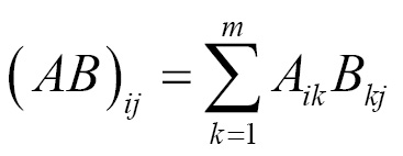
Consider two matrices, A and B, where matrix A has n rows and m columns. Matrix B will have m rows and p columns. The product of A and B, written as AB, is an n row and p column matrix. The m entries of the rows of A are multiplied by the m entries of the columns of matrix B. This is more explicitly shown here, where:
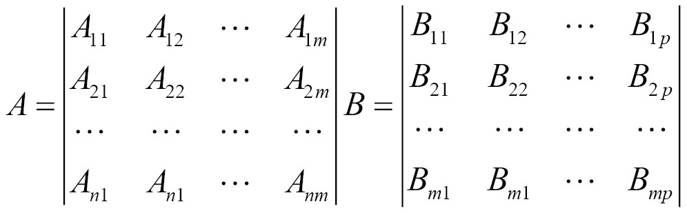
Where the product is defined as follows:
We start with the declaration and initialization of the matrices. The variables n, m, p represent the dimensions of the matrices. The A matrix is n by m, the B matrix is m by p, and the C matrix representing the product is n by p:
int n = 4;
int m = 2;
int p = 3;
double A[][] = {
{0.1950, 0.0311},
{0.3588, 0.2203},
{0.1716, 0.5931},
{0.2105, 0.3242}};
double B[][] = {
{0.0502, 0.9823, 0.9472},
{0.5732, 0.2694, 0.916}};
double C[][] = new double[n][p];
The following code sequence illustrates the multiplication operation using nested for loops:
for (int i = 0; i < n; i++) {
for (int k = 0; k < m; k++) {
for (int j = 0; j < p; j++) {
C[i][j] += A[i][k] * B[k][j];
}
}
}
This following code sequence formats output to display our matrix:
out.println("\nResult");
for (int i = 0; i < n; i++) {
for (int j = 0; j < p; j++) {
out.printf("%.4f ", C[i][j]);
}
out.println();
}
The result appears as follows:
Result 0.0276 0.1999 0.2132 0.1443 0.4118 0.5417 0.3486 0.3283 0.7058 0.1964 0.2941 0.4964
Later, we will demonstrate several alternative techniques for performing the same operation. Next, we will discuss how to tailor support for multiple processors using DL4J.
DeepLearning4j works with GPUs such as those provided by NVIDIA. There are options available that enable the use of GPUs, specify how many GPUs should be used, and control the use of GPU memory. In this section, we will show how you can use these options. This type of control is often available with other high-level APIs.
DL4J uses n-dimensional arrays for Java (ND4J) (http://nd4j.org/) to perform numerical computations. This is a library that supports n-dimensional array objects and other numerical computations, such as linear algebra and signal processing. It includes support for GPUs and is also integrated with Hadoop and Spark.
A vector is a one-dimensional array of numbers and is used extensively with neural networks. A vector is a type of mathematical structure called a tensor. A tensor is essentially a multidimensional array. We can think of a tensor as an array with three or more dimensions, and each dimension is called a rank.
There is often a need to map a multidimensional set of numbers to a one-dimensional array. This is done by flattening the array using a defined order. For example, with a two-dimensional array many systems will allocate the members of the array in row-column order. This means the first row is added to the vector, followed by the second vector, and then the third, and so forth. We will use this approach in the Using the ND4J API section.
To enable GPU use, the project's POM file needs to be modified. In the properties section of the POM file, the nd4j.backend tag needs to added or modified, as shown here:
<nd4j.backend>nd4j-cuda-7.5-platform</<nd4j.backend>
Models can be trained in parallel using the ParallelWrapper class. The training task is automatically distributed among available CPUs/GPUs. The model is used as an argument to the ParallelWrapper class' Builder constructor, as shown here:
ParallelWrapper parallelWrapper =
new ParallelWrapper.Builder(aModel)
// Builder methods...
.build();
When executed, a copy of the model is used on each GPU. After the number of iterations is specified by the averagingFrequency method, the models are averaged and then the training process continues.
There are various methods that can be used to configure the class, as summarized in the following table:
|
Method |
Purpose |
|
|
Specifies the size of a buffer used to pre-fetch data |
|
|
Specifies the number of workers to be used |
|
|
Various methods to control how averaging is achieved |
The number of workers should be greater than the number of GPUs available.
As with most computations, using a lower precision value will speed up the processing. This can be controlled using the setDTypeForContext method, as shown next. In this case, half precision is specified:
DataTypeUtil.setDTypeForContext(DataBuffer.Type.HALF);
This support and more details regarding optimization techniques can be found at http://deeplearning4j.org/gpu.
Map-reduce is a model for processing large sets of data in a parallel, distributed manner. This model consists of a map method for filtering and sorting data, and a reduce method for summarizing data. The map-reduce framework is effective because it distributes the processing of a dataset across multiple servers, performing mapping and reduction simultaneously on smaller pieces of the data. Map-reduce provides significant performance improvements when implemented in a multi-threaded manner. In this section, we will demonstrate a technique using Apache's Hadoop implementation. In the Using Java 8 to perform map-reduce section, we will discuss techniques for performing map-reduce using Java 8 streams.
Hadoop is a software ecosystem providing support for parallel computing. Map-reduce jobs can be run on Hadoop servers, generally set up as clusters, to significantly improve processing speeds. Hadoop has trackers that run map-reduce operations on nodes within a Hadoop cluster. Each node operates independently and the trackers monitor the progress and integrate the output of each node to generate the final output. The following image can be found at http://www.developer.com/java/data/big-data-tool-map-reduce.html and demonstrates the basic map-reduce model with trackers.
We are going to show you a very simple example of a map-reduce application here. Before we can use Hadoop, we need to download and extract Hadoop application files. The latest versions can be found at http://hadoop.apache.org/releases.html. We are using version 2.7.3 for this demonstration.
You will need to set your JAVA_HOME environment variable. Additionally, Hadoop is intolerant of long file paths and spaces within paths, so make sure you extract Hadoop to the simplest directory structure possible.
We will be working with a sample text file containing information about books. Each line of our tab-delimited file has the book title, author, and page count:
Moby Dick Herman Melville 822 Charlotte's Web E.B. White 189 The Grapes of Wrath John Steinbeck 212 Jane Eyre Charlotte Bronte 299 A Tale of Two Cities Charles Dickens 673 War and Peace Leo Tolstoy 1032 The Great Gatsby F. Scott Fitzgerald 275
We are going to use a map function to extract the title and page count information and then a reduce function to calculate the average page count of the books in our dataset. To begin, create a new class, AveragePageCount. We will create two static classes within AveragePageCount, one to handle the map procedure and one to handle the reduction.
First, we will create the TextMapper class, which will implement the map method. This class inherits from the Mapper class and has two private instance variables, pages and bookTitle. pages is an IntWritable object and bookTitle is a Text object. IntWritable and Text are used because these objects will need to be serialized to a byte stream before they can be transmitted to the servers for processing. These objects take up less space and transfer faster than the comparable int or String objects:
public static class TextMapper
extends Mapper<Object, Text, Text, IntWritable> {
private final IntWritable pages = new IntWritable();
private final Text bookTitle = new Text();
}
Within our TextMapper class we create the map method. This method takes three parameters: the key object, a Text object, bookInfo, and the Context. The key allows the tracker to map each particular object back to the correct job. The bookInfo object contains the text or string data about each book. Context holds information about the entire system and allows the method to report on progress and update values within the system.
Within the map method, we use the split method to break each piece of book information into an array of String objects. We set our bookTitle variable to position 0 of the array and set pages to the value stored in position 2, after parsing it as an integer. We can then write out our book title and page count information through the context and update our entire system:
public void map(Object key, Text bookInfo, Context context)
throws IOException, InterruptedException {
String[] book = bookInfo.toString().split("\t");
bookTitle.set(book[0]);
pages.set(Integer.parseInt(book[2]));
context.write(bookTitle, pages);
}
Next, we will write our AverageReduce class. This class extends the Reducer class and will perform the reduction processes to calculate our average page count. We have created four variables for this class: a FloatWritable object to store our average page count, a float average to hold our temporary average, a float count to count how many books exist in our dataset, and an integer sum to add up the page counts:
public static class AverageReduce
extends Reducer<Text, IntWritable, Text, FloatWritable> {
private final FloatWritable finalAvg = new FloatWritable();
Float average = 0f;
Float count = 0f;
int sum = 0;
}
Within our AverageReduce class we will create the reduce method. This method takes as input a Text key, an Iterable object holding writeable integers representing the page counts, and the Context. We use our iterator to process the page counts and add each to our sum. We then calculate the average and set the value of finalAvg. This information is paired with a Text object label and written to the Context:
public void reduce(Text key, Iterable<IntWritable> pageCnts,
Context context)
throws IOException, InterruptedException {
for (IntWritable cnt : pageCnts) {
sum += cnt.get();
}
count += 1;
average = sum / count;
finalAvg.set(average);
context.write(new Text("Average Page Count = "), finalAvg);
}
We are now ready to create our main method in the same class and execute our map-reduce processes. To do this, we need to create a new Configuration object and a new Job. We then set up the significant classes to use in our application.
public static void main(String[] args) throws Exception {
Configuration con = new Configuration();
Job bookJob = Job.getInstance(con, "Average Page Count");
...
}
We set our main class, AveragePageCount, in the setJarByClass method. We specify our TextMapper and AverageReduce classes using the setMapperClass and setReducerClass methods, respectively. We also specify that our output will have a text-based key and a writeable integer using the setOutputKeyClass and setOutputValueClass methods:
bookJob.setJarByClass(AveragePageCount.class);
bookJob.setMapperClass(TextMapper.class);
bookJob.setReducerClass(AverageReduce.class);
bookJob.setOutputKeyClass(Text.class);
bookJob.setOutputValueClass(IntWritable.class);
Finally, we create new input and output paths using the addInputPath and setOutputPath methods. These methods both take our Job object as the first parameter and a Path object representing our input and output file locations as the second parameter. We then call waitForCompletion. Our application exits once this call returns true:
FileInputFormat.addInputPath(bookJob, new Path("C:/Hadoop/books.txt"));
FileOutputFormat.setOutputPath(bookJob, new
Path("C:/Hadoop/BookOutput"));
if (bookJob.waitForCompletion(true)) {
System.exit(0);
}
To execute the application, open a command prompt and navigate to the directory containing our AveragePageCount.class file. We then use the following command to execute our sample application:
hadoop AveragePageCount
While our task is running, we see updated information about our process output to the screen. A sample of our output is shown as follows:
... File System Counters FILE: Number of bytes read=1132 FILE: Number of bytes written=569686 FILE: Number of read operations=0 FILE: Number of large read operations=0 FILE: Number of write operations=0 Map-Reduce Framework Map input records=7 Map output records=7 Map output bytes=136 Map output materialized bytes=156 Input split bytes=90 Combine input records=0 Combine output records=0 Reduce input groups=7 Reduce shuffle bytes=156 Reduce input records=7 Reduce output records=7 Spilled Records=14 Shuffled Maps =1 Failed Shuffles=0 Merged Map outputs=1 GC time elapsed (ms)=11 Total committed heap usage (bytes)=536870912 Shuffle Errors BAD_ID=0 CONNECTION=0 IO_ERROR=0 WRONG_LENGTH=0 WRONG_MAP=0 WRONG_REDUCE=0 File Input Format Counters Bytes Read=249 File Output Format Counters Bytes Written=216
If we open the BookOutput directory created on our local machine, we find four new files. Use a text editor to open part-r-00000. This file contains information about the average page count as it was calculated using parallel processes. A sample of this output follows:
Average Page Count = 673.0 Average Page Count = 431.0 Average Page Count = 387.0 Average Page Count = 495.75 Average Page Count = 439.0 Average Page Count = 411.66666 Average Page Count = 500.2857
Notice how the average changes as each individual process is combined with the other reduction processes. This has the same effect as calculating the average of the first two books first, then adding in the third book, then the fourth, and so on. The advantage here of course is that the averaging is done in a parallel manner. If we had a huge dataset, we should expect to see a noticeable advantage in execution time. The last line of BookOutput reflects the correct and final average of all seven page counts.
Using Apache's Hadoop to perform map-reduce
We are going to show you a very simple example of a map-reduce application here. Before we can use Hadoop, we need to download and extract Hadoop application files. The latest versions can be found at http://hadoop.apache.org/releases.html. We are using version 2.7.3 for this demonstration.
You will need to set your JAVA_HOME environment variable. Additionally, Hadoop is intolerant of long file paths and spaces within paths, so make sure you extract Hadoop to the simplest directory structure possible.
We will be working with a sample text file containing information about books. Each line of our tab-delimited file has the book title, author, and page count:
Moby Dick Herman Melville 822 Charlotte's Web E.B. White 189 The Grapes of Wrath John Steinbeck 212 Jane Eyre Charlotte Bronte 299 A Tale of Two Cities Charles Dickens 673 War and Peace Leo Tolstoy 1032 The Great Gatsby F. Scott Fitzgerald 275
We are going to use a map function to extract the title and page count information and then a reduce function to calculate the average page count of the books in our dataset. To begin, create a new class, AveragePageCount. We will create two static classes within AveragePageCount, one to handle the map procedure and one to handle the reduction.
First, we will create the TextMapper class, which will implement the map method. This class inherits from the Mapper class and has two private instance variables, pages and bookTitle. pages is an IntWritable object and bookTitle is a Text object. IntWritable and Text are used because these objects will need to be serialized to a byte stream before they can be transmitted to the servers for processing. These objects take up less space and transfer faster than the comparable int or String objects:
public static class TextMapper
extends Mapper<Object, Text, Text, IntWritable> {
private final IntWritable pages = new IntWritable();
private final Text bookTitle = new Text();
}
Within our TextMapper class we create the map method. This method takes three parameters: the key object, a Text object, bookInfo, and the Context. The key allows the tracker to map each particular object back to the correct job. The bookInfo object contains the text or string data about each book. Context holds information about the entire system and allows the method to report on progress and update values within the system.
Within the map method, we use the split method to break each piece of book information into an array of String objects. We set our bookTitle variable to position 0 of the array and set pages to the value stored in position 2, after parsing it as an integer. We can then write out our book title and page count information through the context and update our entire system:
public void map(Object key, Text bookInfo, Context context)
throws IOException, InterruptedException {
String[] book = bookInfo.toString().split("\t");
bookTitle.set(book[0]);
pages.set(Integer.parseInt(book[2]));
context.write(bookTitle, pages);
}
Next, we will write our AverageReduce class. This class extends the Reducer class and will perform the reduction processes to calculate our average page count. We have created four variables for this class: a FloatWritable object to store our average page count, a float average to hold our temporary average, a float count to count how many books exist in our dataset, and an integer sum to add up the page counts:
public static class AverageReduce
extends Reducer<Text, IntWritable, Text, FloatWritable> {
private final FloatWritable finalAvg = new FloatWritable();
Float average = 0f;
Float count = 0f;
int sum = 0;
}
Within our AverageReduce class we will create the reduce method. This method takes as input a Text key, an Iterable object holding writeable integers representing the page counts, and the Context. We use our iterator to process the page counts and add each to our sum. We then calculate the average and set the value of finalAvg. This information is paired with a Text object label and written to the Context:
public void reduce(Text key, Iterable<IntWritable> pageCnts,
Context context)
throws IOException, InterruptedException {
for (IntWritable cnt : pageCnts) {
sum += cnt.get();
}
count += 1;
average = sum / count;
finalAvg.set(average);
context.write(new Text("Average Page Count = "), finalAvg);
}
We are now ready to create our main method in the same class and execute our map-reduce processes. To do this, we need to create a new Configuration object and a new Job. We then set up the significant classes to use in our application.
public static void main(String[] args) throws Exception {
Configuration con = new Configuration();
Job bookJob = Job.getInstance(con, "Average Page Count");
...
}
We set our main class, AveragePageCount, in the setJarByClass method. We specify our TextMapper and AverageReduce classes using the setMapperClass and setReducerClass methods, respectively. We also specify that our output will have a text-based key and a writeable integer using the setOutputKeyClass and setOutputValueClass methods:
bookJob.setJarByClass(AveragePageCount.class);
bookJob.setMapperClass(TextMapper.class);
bookJob.setReducerClass(AverageReduce.class);
bookJob.setOutputKeyClass(Text.class);
bookJob.setOutputValueClass(IntWritable.class);
Finally, we create new input and output paths using the addInputPath and setOutputPath methods. These methods both take our Job object as the first parameter and a Path object representing our input and output file locations as the second parameter. We then call waitForCompletion. Our application exits once this call returns true:
FileInputFormat.addInputPath(bookJob, new Path("C:/Hadoop/books.txt"));
FileOutputFormat.setOutputPath(bookJob, new
Path("C:/Hadoop/BookOutput"));
if (bookJob.waitForCompletion(true)) {
System.exit(0);
}
To execute the application, open a command prompt and navigate to the directory containing our AveragePageCount.class file. We then use the following command to execute our sample application:
hadoop AveragePageCount
While our task is running, we see updated information about our process output to the screen. A sample of our output is shown as follows:
... File System Counters FILE: Number of bytes read=1132 FILE: Number of bytes written=569686 FILE: Number of read operations=0 FILE: Number of large read operations=0 FILE: Number of write operations=0 Map-Reduce Framework Map input records=7 Map output records=7 Map output bytes=136 Map output materialized bytes=156 Input split bytes=90 Combine input records=0 Combine output records=0 Reduce input groups=7 Reduce shuffle bytes=156 Reduce input records=7 Reduce output records=7 Spilled Records=14 Shuffled Maps =1 Failed Shuffles=0 Merged Map outputs=1 GC time elapsed (ms)=11 Total committed heap usage (bytes)=536870912 Shuffle Errors BAD_ID=0 CONNECTION=0 IO_ERROR=0 WRONG_LENGTH=0 WRONG_MAP=0 WRONG_REDUCE=0 File Input Format Counters Bytes Read=249 File Output Format Counters Bytes Written=216
If we open the BookOutput directory created on our local machine, we find four new files. Use a text editor to open part-r-00000. This file contains information about the average page count as it was calculated using parallel processes. A sample of this output follows:
Average Page Count = 673.0 Average Page Count = 431.0 Average Page Count = 387.0 Average Page Count = 495.75 Average Page Count = 439.0 Average Page Count = 411.66666 Average Page Count = 500.2857
Notice how the average changes as each individual process is combined with the other reduction processes. This has the same effect as calculating the average of the first two books first, then adding in the third book, then the fourth, and so on. The advantage here of course is that the averaging is done in a parallel manner. If we had a huge dataset, we should expect to see a noticeable advantage in execution time. The last line of BookOutput reflects the correct and final average of all seven page counts.
Writing the map method
First, we will create the TextMapper class, which will implement the map method. This class inherits from the Mapper class and has two private instance variables, pages and bookTitle. pages is an IntWritable object and bookTitle is a Text object. IntWritable and Text are used because these objects will need to be serialized to a byte stream before they can be transmitted to the servers for processing. These objects take up less space and transfer faster than the comparable int or String objects:
public static class TextMapper
extends Mapper<Object, Text, Text, IntWritable> {
private final IntWritable pages = new IntWritable();
private final Text bookTitle = new Text();
}
Within our TextMapper class we create the map method. This method takes three parameters: the key object, a Text object, bookInfo, and the Context. The key allows the tracker to map each particular object back to the correct job. The bookInfo object contains the text or string data about each book. Context holds information about the entire system and allows the method to report on progress and update values within the system.
Within the map method, we use the split method to break each piece of book information into an array of String objects. We set our bookTitle variable to position 0 of the array and set pages to the value stored in position 2, after parsing it as an integer. We can then write out our book title and page count information through the context and update our entire system:
public void map(Object key, Text bookInfo, Context context)
throws IOException, InterruptedException {
String[] book = bookInfo.toString().split("\t");
bookTitle.set(book[0]);
pages.set(Integer.parseInt(book[2]));
context.write(bookTitle, pages);
}
Next, we will write our AverageReduce class. This class extends the Reducer class and will perform the reduction processes to calculate our average page count. We have created four variables for this class: a FloatWritable object to store our average page count, a float average to hold our temporary average, a float count to count how many books exist in our dataset, and an integer sum to add up the page counts:
public static class AverageReduce
extends Reducer<Text, IntWritable, Text, FloatWritable> {
private final FloatWritable finalAvg = new FloatWritable();
Float average = 0f;
Float count = 0f;
int sum = 0;
}
Within our AverageReduce class we will create the reduce method. This method takes as input a Text key, an Iterable object holding writeable integers representing the page counts, and the Context. We use our iterator to process the page counts and add each to our sum. We then calculate the average and set the value of finalAvg. This information is paired with a Text object label and written to the Context:
public void reduce(Text key, Iterable<IntWritable> pageCnts,
Context context)
throws IOException, InterruptedException {
for (IntWritable cnt : pageCnts) {
sum += cnt.get();
}
count += 1;
average = sum / count;
finalAvg.set(average);
context.write(new Text("Average Page Count = "), finalAvg);
}
We are now ready to create our main method in the same class and execute our map-reduce processes. To do this, we need to create a new Configuration object and a new Job. We then set up the significant classes to use in our application.
public static void main(String[] args) throws Exception {
Configuration con = new Configuration();
Job bookJob = Job.getInstance(con, "Average Page Count");
...
}
We set our main class, AveragePageCount, in the setJarByClass method. We specify our TextMapper and AverageReduce classes using the setMapperClass and setReducerClass methods, respectively. We also specify that our output will have a text-based key and a writeable integer using the setOutputKeyClass and setOutputValueClass methods:
bookJob.setJarByClass(AveragePageCount.class);
bookJob.setMapperClass(TextMapper.class);
bookJob.setReducerClass(AverageReduce.class);
bookJob.setOutputKeyClass(Text.class);
bookJob.setOutputValueClass(IntWritable.class);
Finally, we create new input and output paths using the addInputPath and setOutputPath methods. These methods both take our Job object as the first parameter and a Path object representing our input and output file locations as the second parameter. We then call waitForCompletion. Our application exits once this call returns true:
FileInputFormat.addInputPath(bookJob, new Path("C:/Hadoop/books.txt"));
FileOutputFormat.setOutputPath(bookJob, new
Path("C:/Hadoop/BookOutput"));
if (bookJob.waitForCompletion(true)) {
System.exit(0);
}
To execute the application, open a command prompt and navigate to the directory containing our AveragePageCount.class file. We then use the following command to execute our sample application:
hadoop AveragePageCount
While our task is running, we see updated information about our process output to the screen. A sample of our output is shown as follows:
... File System Counters FILE: Number of bytes read=1132 FILE: Number of bytes written=569686 FILE: Number of read operations=0 FILE: Number of large read operations=0 FILE: Number of write operations=0 Map-Reduce Framework Map input records=7 Map output records=7 Map output bytes=136 Map output materialized bytes=156 Input split bytes=90 Combine input records=0 Combine output records=0 Reduce input groups=7 Reduce shuffle bytes=156 Reduce input records=7 Reduce output records=7 Spilled Records=14 Shuffled Maps =1 Failed Shuffles=0 Merged Map outputs=1 GC time elapsed (ms)=11 Total committed heap usage (bytes)=536870912 Shuffle Errors BAD_ID=0 CONNECTION=0 IO_ERROR=0 WRONG_LENGTH=0 WRONG_MAP=0 WRONG_REDUCE=0 File Input Format Counters Bytes Read=249 File Output Format Counters Bytes Written=216
If we open the BookOutput directory created on our local machine, we find four new files. Use a text editor to open part-r-00000. This file contains information about the average page count as it was calculated using parallel processes. A sample of this output follows:
Average Page Count = 673.0 Average Page Count = 431.0 Average Page Count = 387.0 Average Page Count = 495.75 Average Page Count = 439.0 Average Page Count = 411.66666 Average Page Count = 500.2857
Notice how the average changes as each individual process is combined with the other reduction processes. This has the same effect as calculating the average of the first two books first, then adding in the third book, then the fourth, and so on. The advantage here of course is that the averaging is done in a parallel manner. If we had a huge dataset, we should expect to see a noticeable advantage in execution time. The last line of BookOutput reflects the correct and final average of all seven page counts.
Writing the reduce method
Next, we will write our AverageReduce class. This class extends the Reducer class and will perform the reduction processes to calculate our average page count. We have created four variables for this class: a FloatWritable object to store our average page count, a float average to hold our temporary average, a float count to count how many books exist in our dataset, and an integer sum to add up the page counts:
public static class AverageReduce
extends Reducer<Text, IntWritable, Text, FloatWritable> {
private final FloatWritable finalAvg = new FloatWritable();
Float average = 0f;
Float count = 0f;
int sum = 0;
}
Within our AverageReduce class we will create the reduce method. This method takes as input a Text key, an Iterable object holding writeable integers representing the page counts, and the Context. We use our iterator to process the page counts and add each to our sum. We then calculate the average and set the value of finalAvg. This information is paired with a Text object label and written to the Context:
public void reduce(Text key, Iterable<IntWritable> pageCnts,
Context context)
throws IOException, InterruptedException {
for (IntWritable cnt : pageCnts) {
sum += cnt.get();
}
count += 1;
average = sum / count;
finalAvg.set(average);
context.write(new Text("Average Page Count = "), finalAvg);
}
We are now ready to create our main method in the same class and execute our map-reduce processes. To do this, we need to create a new Configuration object and a new Job. We then set up the significant classes to use in our application.
public static void main(String[] args) throws Exception {
Configuration con = new Configuration();
Job bookJob = Job.getInstance(con, "Average Page Count");
...
}
We set our main class, AveragePageCount, in the setJarByClass method. We specify our TextMapper and AverageReduce classes using the setMapperClass and setReducerClass methods, respectively. We also specify that our output will have a text-based key and a writeable integer using the setOutputKeyClass and setOutputValueClass methods:
bookJob.setJarByClass(AveragePageCount.class);
bookJob.setMapperClass(TextMapper.class);
bookJob.setReducerClass(AverageReduce.class);
bookJob.setOutputKeyClass(Text.class);
bookJob.setOutputValueClass(IntWritable.class);
Finally, we create new input and output paths using the addInputPath and setOutputPath methods. These methods both take our Job object as the first parameter and a Path object representing our input and output file locations as the second parameter. We then call waitForCompletion. Our application exits once this call returns true:
FileInputFormat.addInputPath(bookJob, new Path("C:/Hadoop/books.txt"));
FileOutputFormat.setOutputPath(bookJob, new
Path("C:/Hadoop/BookOutput"));
if (bookJob.waitForCompletion(true)) {
System.exit(0);
}
To execute the application, open a command prompt and navigate to the directory containing our AveragePageCount.class file. We then use the following command to execute our sample application:
hadoop AveragePageCount
While our task is running, we see updated information about our process output to the screen. A sample of our output is shown as follows:
... File System Counters FILE: Number of bytes read=1132 FILE: Number of bytes written=569686 FILE: Number of read operations=0 FILE: Number of large read operations=0 FILE: Number of write operations=0 Map-Reduce Framework Map input records=7 Map output records=7 Map output bytes=136 Map output materialized bytes=156 Input split bytes=90 Combine input records=0 Combine output records=0 Reduce input groups=7 Reduce shuffle bytes=156 Reduce input records=7 Reduce output records=7 Spilled Records=14 Shuffled Maps =1 Failed Shuffles=0 Merged Map outputs=1 GC time elapsed (ms)=11 Total committed heap usage (bytes)=536870912 Shuffle Errors BAD_ID=0 CONNECTION=0 IO_ERROR=0 WRONG_LENGTH=0 WRONG_MAP=0 WRONG_REDUCE=0 File Input Format Counters Bytes Read=249 File Output Format Counters Bytes Written=216
If we open the BookOutput directory created on our local machine, we find four new files. Use a text editor to open part-r-00000. This file contains information about the average page count as it was calculated using parallel processes. A sample of this output follows:
Average Page Count = 673.0 Average Page Count = 431.0 Average Page Count = 387.0 Average Page Count = 495.75 Average Page Count = 439.0 Average Page Count = 411.66666 Average Page Count = 500.2857
Notice how the average changes as each individual process is combined with the other reduction processes. This has the same effect as calculating the average of the first two books first, then adding in the third book, then the fourth, and so on. The advantage here of course is that the averaging is done in a parallel manner. If we had a huge dataset, we should expect to see a noticeable advantage in execution time. The last line of BookOutput reflects the correct and final average of all seven page counts.
Creating and executing a new Hadoop job
We are now ready to create our main method in the same class and execute our map-reduce processes. To do this, we need to create a new Configuration object and a new Job. We then set up the significant classes to use in our application.
public static void main(String[] args) throws Exception {
Configuration con = new Configuration();
Job bookJob = Job.getInstance(con, "Average Page Count");
...
}
We set our main class, AveragePageCount, in the setJarByClass method. We specify our TextMapper and AverageReduce classes using the setMapperClass and setReducerClass methods, respectively. We also specify that our output will have a text-based key and a writeable integer using the setOutputKeyClass and setOutputValueClass methods:
bookJob.setJarByClass(AveragePageCount.class);
bookJob.setMapperClass(TextMapper.class);
bookJob.setReducerClass(AverageReduce.class);
bookJob.setOutputKeyClass(Text.class);
bookJob.setOutputValueClass(IntWritable.class);
Finally, we create new input and output paths using the addInputPath and setOutputPath methods. These methods both take our Job object as the first parameter and a Path object representing our input and output file locations as the second parameter. We then call waitForCompletion. Our application exits once this call returns true:
FileInputFormat.addInputPath(bookJob, new Path("C:/Hadoop/books.txt"));
FileOutputFormat.setOutputPath(bookJob, new
Path("C:/Hadoop/BookOutput"));
if (bookJob.waitForCompletion(true)) {
System.exit(0);
}
To execute the application, open a command prompt and navigate to the directory containing our AveragePageCount.class file. We then use the following command to execute our sample application:
hadoop AveragePageCount
While our task is running, we see updated information about our process output to the screen. A sample of our output is shown as follows:
... File System Counters FILE: Number of bytes read=1132 FILE: Number of bytes written=569686 FILE: Number of read operations=0 FILE: Number of large read operations=0 FILE: Number of write operations=0 Map-Reduce Framework Map input records=7 Map output records=7 Map output bytes=136 Map output materialized bytes=156 Input split bytes=90 Combine input records=0 Combine output records=0 Reduce input groups=7 Reduce shuffle bytes=156 Reduce input records=7 Reduce output records=7 Spilled Records=14 Shuffled Maps =1 Failed Shuffles=0 Merged Map outputs=1 GC time elapsed (ms)=11 Total committed heap usage (bytes)=536870912 Shuffle Errors BAD_ID=0 CONNECTION=0 IO_ERROR=0 WRONG_LENGTH=0 WRONG_MAP=0 WRONG_REDUCE=0 File Input Format Counters Bytes Read=249 File Output Format Counters Bytes Written=216
If we open the BookOutput directory created on our local machine, we find four new files. Use a text editor to open part-r-00000. This file contains information about the average page count as it was calculated using parallel processes. A sample of this output follows:
Average Page Count = 673.0 Average Page Count = 431.0 Average Page Count = 387.0 Average Page Count = 495.75 Average Page Count = 439.0 Average Page Count = 411.66666 Average Page Count = 500.2857
Notice how the average changes as each individual process is combined with the other reduction processes. This has the same effect as calculating the average of the first two books first, then adding in the third book, then the fourth, and so on. The advantage here of course is that the averaging is done in a parallel manner. If we had a huge dataset, we should expect to see a noticeable advantage in execution time. The last line of BookOutput reflects the correct and final average of all seven page counts.
There are numerous mathematical libraries available for Java use. In this section, we will provide a quick and high-level overview of several libraries. These libraries do not necessarily automatically support multiple processors. In addition, the intent of this section is to provide some insight into how these libraries can be used. In most cases, they are relatively easy to use.
A list of Java mathematical libraries is found at https://en.wikipedia.org/wiki/List_of_numerical_libraries#Java and https://java-matrix.org/. We will demonstrate the use of the jblas, Apache Commons Math, and the ND4J libraries.
The jblas API (http://jblas.org/) is a math library supporting Java. It is based on Basic Linear Algebra Subprograms (BLAS) (http://www.netlib.org/blas/) and Linear Algebra Package (LAPACK) (http://www.netlib.org/lapack/), which are standard libraries for fast arithmetic calculation. The jblas API provides a wrapper around these libraries.
The following is a demonstration of how matrix multiplication is performed. We start with the matrix definitions:
DoubleMatrix A = new DoubleMatrix(new double[][]{
{0.1950, 0.0311},
{0.3588, 0.2203},
{0.1716, 0.5931},
{0.2105, 0.3242}});
DoubleMatrix B = new DoubleMatrix(new double[][]{
{0.0502, 0.9823, 0.9472},
{0.5732, 0.2694, 0.916}});
DoubleMatrix C;
The actual statement to perform multiplication is quite short, as shown next. The mmul method is executed against the A matrix, where the B array is passed as an argument:
C = A.mmul(B);
The resulting C matrix is then displayed:
for(int i=0; i<C.getRows(); i++) {
out.println(C.getRow(i));
}
The output should be as follows:
[0.027616, 0.199927, 0.213192] [0.144288, 0.411798, 0.541650] [0.348579, 0.328344, 0.705819] [0.196399, 0.294114, 0.496353]
This library is fairly easy to use and supports an extensive set of arithmetic operations.
The Apache Commons math API (http://commons.apache.org/proper/commons-math/) supports a large number of mathematical and statistical operations. The following example illustrates how to perform matrix multiplication.
We start with the declaration and initialization of the A and B matrices:
double[][] A = {
{0.1950, 0.0311},
{0.3588, 0.2203},
{0.1716, 0.5931},
{0.2105, 0.3242}};
double[][] B = {
{0.0502, 0.9823, 0.9472},
{0.5732, 0.2694, 0.916}};
Apache Commons uses the RealMatrix class to hold a matrix. In the following code sequence, the corresponding matrices for the A and B matrices are created using the Array2DRowRealMatrix constructor:
RealMatrix aRealMatrix = new Array2DRowRealMatrix(A); RealMatrix bRealMatrix = new Array2DRowRealMatrix(B);
The multiplication is straightforward using the multiply method, as shown next:
RealMatrix cRealMatrix = aRealMatrix.multiply(bRealMatrix);
The next for loop will display the following results:
for (int i = 0; i < cRealMatrix.getRowDimension(); i++) {
out.println(cRealMatrix.getRowVector(i));
}
The output should be as follows:
{0.02761552; 0.19992684; 0.2131916} {0.14428772; 0.41179806; 0.54165016} {0.34857924; 0.32834382; 0.70581912} {0.19639854; 0.29411363; 0.4963528}
ND4J (http://nd4j.org/) is the library used by DL4J to perform arithmetic operations. The library is also available for direct use. In this section, we will demonstrate how matrix multiplication is performed using the A and B matrices.
Before we can perform the multiplication, we need to flatten the matrices to vectors. The following declares and initializes these vectors:
double[] A = {
0.1950, 0.0311,
0.3588, 0.2203,
0.1716, 0.5931,
0.2105, 0.3242};
double[] B = {
0.0502, 0.9823, 0.9472,
0.5732, 0.2694, 0.916};
The Nd4j class' create method creates an INDArray instance given a vector and dimension information. The first argument of the method is the vector. The second argument specifies the dimensions of the matrix. The last argument specifies the order the rows and columns are laid out. This order is either row-column major as exemplified by c, or column-row major order as used by FORTRAN. Row-column order means the first row is allocated to the vector, followed by the second row, and so forth.
In the following code sequence 2INDArray instances are created using the A and B vectors. The first is a 4 row, 2 column matrix using row-major order as specified by the third argument, c. The second INDArray instance represents the B matrix. If we wanted to use column-row ordering, we would use an f instead.
INDArray aINDArray = Nd4j.create(A,new int[]{4,2},'c');
INDArray bINDArray = Nd4j.create(B,new int[]{2,3},'c');
The C array, represented by cINDArray, is then declared and assigned the result of the multiplication. The mmul performs the operation:
INDArray cINDArray; cINDArray = aINDArray.mmul(bINDArray);
The following sequence displays the results using the getRow method:
for(int i=0; i<cINDArray.rows(); i++) {
out.println(cINDArray.getRow(i));
}
The output should be as follows:
[0.03, 0.20, 0.21] [0.14, 0.41, 0.54] [0.35, 0.33, 0.71] [0.20, 0.29, 0.50]
Next, we will provide an overview of the OpenCL API that provide supports for concurrent operations on a number of platforms.
Using the jblas API
The jblas API (http://jblas.org/) is a math library supporting Java. It is based on Basic Linear Algebra Subprograms (BLAS) (http://www.netlib.org/blas/) and Linear Algebra Package (LAPACK) (http://www.netlib.org/lapack/), which are standard libraries for fast arithmetic calculation. The jblas API provides a wrapper around these libraries.
The following is a demonstration of how matrix multiplication is performed. We start with the matrix definitions:
DoubleMatrix A = new DoubleMatrix(new double[][]{
{0.1950, 0.0311},
{0.3588, 0.2203},
{0.1716, 0.5931},
{0.2105, 0.3242}});
DoubleMatrix B = new DoubleMatrix(new double[][]{
{0.0502, 0.9823, 0.9472},
{0.5732, 0.2694, 0.916}});
DoubleMatrix C;
The actual statement to perform multiplication is quite short, as shown next. The mmul method is executed against the A matrix, where the B array is passed as an argument:
C = A.mmul(B);
The resulting C matrix is then displayed:
for(int i=0; i<C.getRows(); i++) {
out.println(C.getRow(i));
}
The output should be as follows:
[0.027616, 0.199927, 0.213192] [0.144288, 0.411798, 0.541650] [0.348579, 0.328344, 0.705819] [0.196399, 0.294114, 0.496353]
This library is fairly easy to use and supports an extensive set of arithmetic operations.
The Apache Commons math API (http://commons.apache.org/proper/commons-math/) supports a large number of mathematical and statistical operations. The following example illustrates how to perform matrix multiplication.
We start with the declaration and initialization of the A and B matrices:
double[][] A = {
{0.1950, 0.0311},
{0.3588, 0.2203},
{0.1716, 0.5931},
{0.2105, 0.3242}};
double[][] B = {
{0.0502, 0.9823, 0.9472},
{0.5732, 0.2694, 0.916}};
Apache Commons uses the RealMatrix class to hold a matrix. In the following code sequence, the corresponding matrices for the A and B matrices are created using the Array2DRowRealMatrix constructor:
RealMatrix aRealMatrix = new Array2DRowRealMatrix(A); RealMatrix bRealMatrix = new Array2DRowRealMatrix(B);
The multiplication is straightforward using the multiply method, as shown next:
RealMatrix cRealMatrix = aRealMatrix.multiply(bRealMatrix);
The next for loop will display the following results:
for (int i = 0; i < cRealMatrix.getRowDimension(); i++) {
out.println(cRealMatrix.getRowVector(i));
}
The output should be as follows:
{0.02761552; 0.19992684; 0.2131916} {0.14428772; 0.41179806; 0.54165016} {0.34857924; 0.32834382; 0.70581912} {0.19639854; 0.29411363; 0.4963528}
ND4J (http://nd4j.org/) is the library used by DL4J to perform arithmetic operations. The library is also available for direct use. In this section, we will demonstrate how matrix multiplication is performed using the A and B matrices.
Before we can perform the multiplication, we need to flatten the matrices to vectors. The following declares and initializes these vectors:
double[] A = {
0.1950, 0.0311,
0.3588, 0.2203,
0.1716, 0.5931,
0.2105, 0.3242};
double[] B = {
0.0502, 0.9823, 0.9472,
0.5732, 0.2694, 0.916};
The Nd4j class' create method creates an INDArray instance given a vector and dimension information. The first argument of the method is the vector. The second argument specifies the dimensions of the matrix. The last argument specifies the order the rows and columns are laid out. This order is either row-column major as exemplified by c, or column-row major order as used by FORTRAN. Row-column order means the first row is allocated to the vector, followed by the second row, and so forth.
In the following code sequence 2INDArray instances are created using the A and B vectors. The first is a 4 row, 2 column matrix using row-major order as specified by the third argument, c. The second INDArray instance represents the B matrix. If we wanted to use column-row ordering, we would use an f instead.
INDArray aINDArray = Nd4j.create(A,new int[]{4,2},'c');
INDArray bINDArray = Nd4j.create(B,new int[]{2,3},'c');
The C array, represented by cINDArray, is then declared and assigned the result of the multiplication. The mmul performs the operation:
INDArray cINDArray; cINDArray = aINDArray.mmul(bINDArray);
The following sequence displays the results using the getRow method:
for(int i=0; i<cINDArray.rows(); i++) {
out.println(cINDArray.getRow(i));
}
The output should be as follows:
[0.03, 0.20, 0.21] [0.14, 0.41, 0.54] [0.35, 0.33, 0.71] [0.20, 0.29, 0.50]
Next, we will provide an overview of the OpenCL API that provide supports for concurrent operations on a number of platforms.
Using the Apache Commons math API
The Apache Commons math API (http://commons.apache.org/proper/commons-math/) supports a large number of mathematical and statistical operations. The following example illustrates how to perform matrix multiplication.
We start with the declaration and initialization of the A and B matrices:
double[][] A = {
{0.1950, 0.0311},
{0.3588, 0.2203},
{0.1716, 0.5931},
{0.2105, 0.3242}};
double[][] B = {
{0.0502, 0.9823, 0.9472},
{0.5732, 0.2694, 0.916}};
Apache Commons uses the RealMatrix class to hold a matrix. In the following code sequence, the corresponding matrices for the A and B matrices are created using the Array2DRowRealMatrix constructor:
RealMatrix aRealMatrix = new Array2DRowRealMatrix(A); RealMatrix bRealMatrix = new Array2DRowRealMatrix(B);
The multiplication is straightforward using the multiply method, as shown next:
RealMatrix cRealMatrix = aRealMatrix.multiply(bRealMatrix);
The next for loop will display the following results:
for (int i = 0; i < cRealMatrix.getRowDimension(); i++) {
out.println(cRealMatrix.getRowVector(i));
}
The output should be as follows:
{0.02761552; 0.19992684; 0.2131916} {0.14428772; 0.41179806; 0.54165016} {0.34857924; 0.32834382; 0.70581912} {0.19639854; 0.29411363; 0.4963528}
ND4J (http://nd4j.org/) is the library used by DL4J to perform arithmetic operations. The library is also available for direct use. In this section, we will demonstrate how matrix multiplication is performed using the A and B matrices.
Before we can perform the multiplication, we need to flatten the matrices to vectors. The following declares and initializes these vectors:
double[] A = {
0.1950, 0.0311,
0.3588, 0.2203,
0.1716, 0.5931,
0.2105, 0.3242};
double[] B = {
0.0502, 0.9823, 0.9472,
0.5732, 0.2694, 0.916};
The Nd4j class' create method creates an INDArray instance given a vector and dimension information. The first argument of the method is the vector. The second argument specifies the dimensions of the matrix. The last argument specifies the order the rows and columns are laid out. This order is either row-column major as exemplified by c, or column-row major order as used by FORTRAN. Row-column order means the first row is allocated to the vector, followed by the second row, and so forth.
In the following code sequence 2INDArray instances are created using the A and B vectors. The first is a 4 row, 2 column matrix using row-major order as specified by the third argument, c. The second INDArray instance represents the B matrix. If we wanted to use column-row ordering, we would use an f instead.
INDArray aINDArray = Nd4j.create(A,new int[]{4,2},'c');
INDArray bINDArray = Nd4j.create(B,new int[]{2,3},'c');
The C array, represented by cINDArray, is then declared and assigned the result of the multiplication. The mmul performs the operation:
INDArray cINDArray; cINDArray = aINDArray.mmul(bINDArray);
The following sequence displays the results using the getRow method:
for(int i=0; i<cINDArray.rows(); i++) {
out.println(cINDArray.getRow(i));
}
The output should be as follows:
[0.03, 0.20, 0.21] [0.14, 0.41, 0.54] [0.35, 0.33, 0.71] [0.20, 0.29, 0.50]
Next, we will provide an overview of the OpenCL API that provide supports for concurrent operations on a number of platforms.
Using the ND4J API
ND4J (http://nd4j.org/) is the library used by DL4J to perform arithmetic operations. The library is also available for direct use. In this section, we will demonstrate how matrix multiplication is performed using the A and B matrices.
Before we can perform the multiplication, we need to flatten the matrices to vectors. The following declares and initializes these vectors:
double[] A = {
0.1950, 0.0311,
0.3588, 0.2203,
0.1716, 0.5931,
0.2105, 0.3242};
double[] B = {
0.0502, 0.9823, 0.9472,
0.5732, 0.2694, 0.916};
The Nd4j class' create method creates an INDArray instance given a vector and dimension information. The first argument of the method is the vector. The second argument specifies the dimensions of the matrix. The last argument specifies the order the rows and columns are laid out. This order is either row-column major as exemplified by c, or column-row major order as used by FORTRAN. Row-column order means the first row is allocated to the vector, followed by the second row, and so forth.
In the following code sequence 2INDArray instances are created using the A and B vectors. The first is a 4 row, 2 column matrix using row-major order as specified by the third argument, c. The second INDArray instance represents the B matrix. If we wanted to use column-row ordering, we would use an f instead.
INDArray aINDArray = Nd4j.create(A,new int[]{4,2},'c');
INDArray bINDArray = Nd4j.create(B,new int[]{2,3},'c');
The C array, represented by cINDArray, is then declared and assigned the result of the multiplication. The mmul performs the operation:
INDArray cINDArray; cINDArray = aINDArray.mmul(bINDArray);
The following sequence displays the results using the getRow method:
for(int i=0; i<cINDArray.rows(); i++) {
out.println(cINDArray.getRow(i));
}
The output should be as follows:
[0.03, 0.20, 0.21] [0.14, 0.41, 0.54] [0.35, 0.33, 0.71] [0.20, 0.29, 0.50]
Next, we will provide an overview of the OpenCL API that provide supports for concurrent operations on a number of platforms.
Open Computing Language (OpenCL) (https://www.khronos.org/opencl/) supports programs that execute across heterogeneous platforms, that is, platforms potentially using different vendors and architectures. The platforms can use different processing units, including Central Processing Unit (CPU), Graphical Processing Unit (GPU), Digital Signal Processor (DSP), Field-Programmable Gate Array (FPGA), and other types of processors.
OpenCL uses a C99-based language to program the devices, providing a standard interface for programming concurrent behavior. OpenCL supports an API that allows code to be written in different languages. For Java, there are several APIs that support the development of OpenCL based languages:
- Java bindings for OpenCL (JOCL) (http://www.jocl.org/) - This is a binding to the original OpenCL C implementation and can be verbose.
- JavaCl (https://code.google.com/archive/p/javacl/) - Provides an object-oriented interface to JOCL.
- Java OpenCL (http://jogamp.org/jocl/www/) - Also provides an object-oriented abstraction of JOCL. It is not intended for client use.
- The Lightweight Java Game Library (LWJGL) (https://www.lwjgl.org/) - Also provides support for OpenCL and is oriented toward GUI applications.
In addition, Aparapi provides higher-level access to OpenCL, thus avoiding some of the complexity involved in creating OpenCL applications.
Code that runs on a processor is encapsulated in a kernel. Multiple kernels will execute in parallel on different computing devices. There are different levels of memory supported by OpenCL. A specific device may not support each level. The levels include:
- Global memory - Shared by all computing units
- Read-only memory - Generally not writable
- Local memory - Shared by a group of computing units
- Per-element private memory - Often a register
OpenCL applications require a considerable amount of initial code to be useful. This complexity does not permit us to provide a detailed example of its use. However, the Aparapi section does provide some feel for how OpenCL applications are structured.
Aparapi (https://github.com/aparapi/aparapi) is a Java library that supports concurrent operations. The API supports code running on GPUs or CPUs. GPU operations are executed using OpenCL, while CPU operations use Java threads. The user can specify which computing resource to use. However, if GPU support is not available, Aparapi will revert to Java threads.
The API will convert Java byte codes to OpenCL at runtime. This makes the API largely independent from the graphics card used. The API was initially developed by AMD but has been released as open source. This is reflected in the basic package name, com.amd.aparari. Aparapi offers a higher level of abstraction than provided by OpenCL.
Aparapi code is located in a class derived from the Kernel class. Its execute method will start the operations. This will result in an internal call to a run method, which needs to be overridden. It is within the run method that concurrent code is placed. The run method is executed multiple times on different processors.
Due to OpenCL limitations, we are unable to use inheritance or method overloading. In addition, it does not like println in the run method, since the code may be running on a GPI. Aparapi only supports one-dimensional arrays. Arrays using two or more dimensions need to be flattened to a one dimension array. The support for double values is dependent on the OpenCL version and GPU configuration.
When a Java thread pool is used, it allocates one thread per CPU core. The kernel containing the Java code is cloned, one copy per thread. This avoids the need to access data across a thread. Each thread has access to information, such as a global ID, to assist in the code execution. The kernel will wait for all of the threads to complete.
Aparapi downloads can be found at https://github.com/aparapi/aparapi/releases.
The basic framework for an Aparapi application is shown next. It consists of a Kernel derived class where the run method is overridden. In this example, the run method will perform scalar multiplication. This operation involves multiplying each element of a vector by some value.
The ScalarMultiplicationKernel extends the Kernel class. It possesses two instance variables used to hold the matrices for input and output. The constructor will initialize the matrices. The run method will perform the actual computations, and the displayResult method will show the results of the multiplication:
public class ScalarMultiplicationKernel extends Kernel {
float[] inputMatrix;
float outputMatrix [];
public ScalarMultiplicationKernel(float inputMatrix[]) {
...
}
@Override
public void run() {
...
}
public void displayResult() {
...
}
}
The constructor is shown here:
public ScalarMultiplicationKernel(float inputMatrix[]) {
this.inputMatrix = inputMatrix;
outputMatrix = new float[this.inputMatrix.length];
}
In the run method, we use a global ID to index into the matrix. This code is executed on each computation unit, for example, a GPU or thread. A unique global ID is provided to each computational unit, allowing the code to access a specific element of the matrix. In this example, each element of the input matrix is multiplied by 2 and then assigned to the corresponding element of the output matrix:
public void run() {
int globalID = this.getGlobalId();
outputMatrix[globalID] = 2.0f * inputMatrix[globalID];
}
The displayResult method simply displays the contents of the outputMatrix array:
public void displayResult() {
out.println("Result");
for (float element : outputMatrix) {
out.printf("%.4f ", element);
}
out.println();
}
To use this kernel, we need to declare variables for the inputMatrix and its size. The size will be used to control how many kernels to execute:
float inputMatrix[] = {3, 4, 5, 6, 7, 8, 9};
int size = inputMatrix.length;
The kernel is then created using the input matrix followed by the invocation of the execute method. This method starts the process and will eventually invoke the Kernel class' run method based on the execute method's argument. This argument is referred to as the pass ID. While not used in this example, we will use it in the next section. When the process is complete, the resulting output matrix is displayed and the dispose method is called to stop the process:
ScalarMultiplicationKernel kernel =
new ScalarMultiplicationKernel(inputMatrix);
kernel.execute(size);
kernel.displayResult();
kernel.dispose();
When this application is executed we will get the following output:
6.0000 8.0000 10.0000 12.0000 14.0000 16.0000 18.000
We can specify the execution mode using the Kernel class' setExecutionMode method, as shown here:
kernel.setExecutionMode(Kernel.EXECUTION_MODE.GPU);
However, it is best to let Aparapi determine the execution mode. The following table summarizes the execution modes available:
|
Execution mode |
Meaning |
|
|
Does not specify mode |
|
|
Use CPU |
|
|
Use GPU |
|
|
Use Java threads |
|
|
Use single loop (for debugging purposes) |
Next, we will demonstrate how we can use Aparapi to perform dot product matrix multiplication.
We will use the matrices as used in the Implementing basic matrix operations section. We start with the declaration of the MatrixMultiplicationKernel class, which contains the vector declarations, a constructor, the run method, and a displayResults method. The vectors for matrices A and B have been flattened to one-dimensional arrays by allocating the matrices in row-column order:
class MatrixMultiplicationKernel extends Kernel {
float[] vectorA = {
0.1950f, 0.0311f, 0.3588f,
0.2203f, 0.1716f, 0.5931f,
0.2105f, 0.3242f};
float[] vectorB = {
0.0502f, 0.9823f, 0.9472f,
0.5732f, 0.2694f, 0.916f};
float[] vectorC;
int n;
int m;
int p;
@Override
public void run() {
...
}
public MatrixMultiplicationKernel(int n, int m, int p) {
...
}
public void displayResults () {
...
}
}
The MatrixMultiplicationKernel constructor assigns values for the matrices' dimensions and allocates memory for the result stored in vectorC, as shown here:
public MatrixMultiplicationKernel(int n, int m, int p) {
this.n = n;
this.p = p;
this.m = m;
vectorC = new float[n * p];
}
The run method uses a global ID and a pass ID to perform the matrix multiplication. The pass ID is specified as the second argument of the Kernel class' execute method, as we will see shortly. This value allows us to advance the column index for vectorC. The vector indexes map to the corresponding row and column positions of the original matrices:
public void run() {
int i = getGlobalId();
int j = this.getPassId();
float value = 0;
for (int k = 0; k < p; k++) {
value += vectorA[k + i * m] * vectorB[k * p + j];
}
vectorC[i * p + j] = value;
}
The displayResults method is shown as follows:
public void displayResults() {
out.println("Result");
for (int i = 0; i < n; i++) {
for (int j = 0; j < p; j++) {
out.printf("%.4f ", vectorC[i * p + j]);
}
out.println();
}
}
The kernel is started in the same way as in the previous section. The execute method is passed the number of kernels that should be created and an integer indicating the number of passes to make. The number of passes is used to control the index into the vectorA and vectorB arrays:
MatrixMultiplicationKernel kernel = new MatrixMultiplicationKernel(n, m, p);kernel.execute(6, 3);kernel.displayResults(); kernel.dispose();
When this example is executed, you will get the following output:
Result 0.0276 0.1999 0.2132 0.1443 0.4118 0.5417 0.3486 0.3283 0.7058 0.1964 0.2941 0.4964
Next, we will see how Java 8 additions can contribute to solving math-intensive problems in a parallel manner.
Creating an Aparapi application
The basic framework for an Aparapi application is shown next. It consists of a Kernel derived class where the run method is overridden. In this example, the run method will perform scalar multiplication. This operation involves multiplying each element of a vector by some value.
The ScalarMultiplicationKernel extends the Kernel class. It possesses two instance variables used to hold the matrices for input and output. The constructor will initialize the matrices. The run method will perform the actual computations, and the displayResult method will show the results of the multiplication:
public class ScalarMultiplicationKernel extends Kernel {
float[] inputMatrix;
float outputMatrix [];
public ScalarMultiplicationKernel(float inputMatrix[]) {
...
}
@Override
public void run() {
...
}
public void displayResult() {
...
}
}
The constructor is shown here:
public ScalarMultiplicationKernel(float inputMatrix[]) {
this.inputMatrix = inputMatrix;
outputMatrix = new float[this.inputMatrix.length];
}
In the run method, we use a global ID to index into the matrix. This code is executed on each computation unit, for example, a GPU or thread. A unique global ID is provided to each computational unit, allowing the code to access a specific element of the matrix. In this example, each element of the input matrix is multiplied by 2 and then assigned to the corresponding element of the output matrix:
public void run() {
int globalID = this.getGlobalId();
outputMatrix[globalID] = 2.0f * inputMatrix[globalID];
}
The displayResult method simply displays the contents of the outputMatrix array:
public void displayResult() {
out.println("Result");
for (float element : outputMatrix) {
out.printf("%.4f ", element);
}
out.println();
}
To use this kernel, we need to declare variables for the inputMatrix and its size. The size will be used to control how many kernels to execute:
float inputMatrix[] = {3, 4, 5, 6, 7, 8, 9};
int size = inputMatrix.length;
The kernel is then created using the input matrix followed by the invocation of the execute method. This method starts the process and will eventually invoke the Kernel class' run method based on the execute method's argument. This argument is referred to as the pass ID. While not used in this example, we will use it in the next section. When the process is complete, the resulting output matrix is displayed and the dispose method is called to stop the process:
ScalarMultiplicationKernel kernel =
new ScalarMultiplicationKernel(inputMatrix);
kernel.execute(size);
kernel.displayResult();
kernel.dispose();
When this application is executed we will get the following output:
6.0000 8.0000 10.0000 12.0000 14.0000 16.0000 18.000
We can specify the execution mode using the Kernel class' setExecutionMode method, as shown here:
kernel.setExecutionMode(Kernel.EXECUTION_MODE.GPU);
However, it is best to let Aparapi determine the execution mode. The following table summarizes the execution modes available:
|
Execution mode |
Meaning |
|
|
Does not specify mode |
|
|
Use CPU |
|
|
Use GPU |
|
|
Use Java threads |
|
|
Use single loop (for debugging purposes) |
Next, we will demonstrate how we can use Aparapi to perform dot product matrix multiplication.
We will use the matrices as used in the Implementing basic matrix operations section. We start with the declaration of the MatrixMultiplicationKernel class, which contains the vector declarations, a constructor, the run method, and a displayResults method. The vectors for matrices A and B have been flattened to one-dimensional arrays by allocating the matrices in row-column order:
class MatrixMultiplicationKernel extends Kernel {
float[] vectorA = {
0.1950f, 0.0311f, 0.3588f,
0.2203f, 0.1716f, 0.5931f,
0.2105f, 0.3242f};
float[] vectorB = {
0.0502f, 0.9823f, 0.9472f,
0.5732f, 0.2694f, 0.916f};
float[] vectorC;
int n;
int m;
int p;
@Override
public void run() {
...
}
public MatrixMultiplicationKernel(int n, int m, int p) {
...
}
public void displayResults () {
...
}
}
The MatrixMultiplicationKernel constructor assigns values for the matrices' dimensions and allocates memory for the result stored in vectorC, as shown here:
public MatrixMultiplicationKernel(int n, int m, int p) {
this.n = n;
this.p = p;
this.m = m;
vectorC = new float[n * p];
}
The run method uses a global ID and a pass ID to perform the matrix multiplication. The pass ID is specified as the second argument of the Kernel class' execute method, as we will see shortly. This value allows us to advance the column index for vectorC. The vector indexes map to the corresponding row and column positions of the original matrices:
public void run() {
int i = getGlobalId();
int j = this.getPassId();
float value = 0;
for (int k = 0; k < p; k++) {
value += vectorA[k + i * m] * vectorB[k * p + j];
}
vectorC[i * p + j] = value;
}
The displayResults method is shown as follows:
public void displayResults() {
out.println("Result");
for (int i = 0; i < n; i++) {
for (int j = 0; j < p; j++) {
out.printf("%.4f ", vectorC[i * p + j]);
}
out.println();
}
}
The kernel is started in the same way as in the previous section. The execute method is passed the number of kernels that should be created and an integer indicating the number of passes to make. The number of passes is used to control the index into the vectorA and vectorB arrays:
MatrixMultiplicationKernel kernel = new MatrixMultiplicationKernel(n, m, p);kernel.execute(6, 3);kernel.displayResults(); kernel.dispose();
When this example is executed, you will get the following output:
Result 0.0276 0.1999 0.2132 0.1443 0.4118 0.5417 0.3486 0.3283 0.7058 0.1964 0.2941 0.4964
Next, we will see how Java 8 additions can contribute to solving math-intensive problems in a parallel manner.
Using Aparapi for matrix multiplication
We will use the matrices as used in the Implementing basic matrix operations section. We start with the declaration of the MatrixMultiplicationKernel class, which contains the vector declarations, a constructor, the run method, and a displayResults method. The vectors for matrices A and B have been flattened to one-dimensional arrays by allocating the matrices in row-column order:
class MatrixMultiplicationKernel extends Kernel {
float[] vectorA = {
0.1950f, 0.0311f, 0.3588f,
0.2203f, 0.1716f, 0.5931f,
0.2105f, 0.3242f};
float[] vectorB = {
0.0502f, 0.9823f, 0.9472f,
0.5732f, 0.2694f, 0.916f};
float[] vectorC;
int n;
int m;
int p;
@Override
public void run() {
...
}
public MatrixMultiplicationKernel(int n, int m, int p) {
...
}
public void displayResults () {
...
}
}
The MatrixMultiplicationKernel constructor assigns values for the matrices' dimensions and allocates memory for the result stored in vectorC, as shown here:
public MatrixMultiplicationKernel(int n, int m, int p) {
this.n = n;
this.p = p;
this.m = m;
vectorC = new float[n * p];
}
The run method uses a global ID and a pass ID to perform the matrix multiplication. The pass ID is specified as the second argument of the Kernel class' execute method, as we will see shortly. This value allows us to advance the column index for vectorC. The vector indexes map to the corresponding row and column positions of the original matrices:
public void run() {
int i = getGlobalId();
int j = this.getPassId();
float value = 0;
for (int k = 0; k < p; k++) {
value += vectorA[k + i * m] * vectorB[k * p + j];
}
vectorC[i * p + j] = value;
}
The displayResults method is shown as follows:
public void displayResults() {
out.println("Result");
for (int i = 0; i < n; i++) {
for (int j = 0; j < p; j++) {
out.printf("%.4f ", vectorC[i * p + j]);
}
out.println();
}
}
The kernel is started in the same way as in the previous section. The execute method is passed the number of kernels that should be created and an integer indicating the number of passes to make. The number of passes is used to control the index into the vectorA and vectorB arrays:
MatrixMultiplicationKernel kernel = new MatrixMultiplicationKernel(n, m, p);kernel.execute(6, 3);kernel.displayResults(); kernel.dispose();
When this example is executed, you will get the following output:
Result 0.0276 0.1999 0.2132 0.1443 0.4118 0.5417 0.3486 0.3283 0.7058 0.1964 0.2941 0.4964
Next, we will see how Java 8 additions can contribute to solving math-intensive problems in a parallel manner.
The release of Java 8 came with a number of important enhancements to the language. The two enhancements of interest to us include lambda expressions and streams. A lambda expression is essentially an anonymous function that adds a functional programming dimension to Java. The concept of streams, as introduced in Java 8, does not refer to IO streams. Instead, you can think of it as a sequence of objects that can be generated and manipulated using a fluent style of programming. This style will be demonstrated shortly.
As with most APIs, programmers must be careful to consider the actual execution performance of their code using realistic test cases and environments. If not used properly, streams may not actually provide performance improvements. In particular, parallel streams, if not crafted carefully, can produce incorrect results.
We will start with a quick introduction to lambda expressions and streams. If you are familiar with these concepts you may want to skip over the next section.
A lambda expression can be expressed in several different forms. The following illustrates a simple lambda expression where the symbol, ->, is the lambda operator. This will take some value, e, and return the value multiplied by two. There is nothing special about the name e. Any valid Java variable name can be used:
e -> 2 * e
It can also be expressed in other forms, such as the following:
(int e) -> 2 * e
(double e) -> 2 * e
(int e) -> {return 2 * e;
The form used depends on the intended value of e. Lambda expressions are frequently used as arguments to a method, as we will see shortly.
A stream can be created using a number of techniques. In the following example, a stream is created from an array. The IntStream interface is a type of stream that uses integers. The Arrays class' stream method converts an array into a stream:
IntStream stream = Arrays.stream(numbers);
We can then apply various stream methods to perform an operation. In the following statement, the forEach method will simply display each integer in the stream:
stream.forEach(e -> out.printf("%d ", e));
There are a variety of stream methods that can be applied to a stream. In the following example, the mapToDouble method will take an integer, multiply it by 2, and then return it as a double. The forEach method will then display these values:
stream
.mapToDouble(e-> 2 * e)
.forEach(e -> out.printf("%.4f ", e));
The cascading of method invocations is referred to as fluent programing.
Here, we will illustrate how streams can be used to perform matrix multiplication. The definitions of the A, B, and C matrices are the same as declared in the Implementing basic matrix operations section. They are duplicated here for your convenience:
double A[][] = {
{0.1950, 0.0311},
{0.3588, 0.2203},
{0.1716, 0.5931},
{0.2105, 0.3242}};
double B[][] = {
{0.0502, 0.9823, 0.9472},
{0.5732, 0.2694, 0.916}};
double C[][] = new double[n][p];
The following sequence is a stream implementation of matrix multiplication. A detailed explanation of the code follows:
C = Arrays.stream(A)
.parallel()
.map(AMatrixRow -> IntStream.range(0, B[0].length)
.mapToDouble(i -> IntStream.range(0, B.length)
.mapToDouble(j -> AMatrixRow[j] * B[j][i])
.sum()
).toArray()).toArray(double[][]::new);
The first map method, shown as follows, creates a stream of double vectors representing the 4 rows of the A matrix. The range method will return a list of stream elements ranging from its first argument to the second argument.
.map(AMatrixRow -> IntStream.range(0, B[0].length)
The variable i corresponds to the numbers generated by the second range method, which corresponds to the number of rows in the B matrix (2). The variable j corresponds to the numbers generated by the third range method, representing the number of columns of the B matrix (3).
At the heart of the statement is the matrix multiplication, where the sum method calculates the sum:
.mapToDouble(j -> AMatrixRow[j] * B[j][i]) .sum()
The last part of the expression creates the two-dimensional array for the C matrix. The operator, ::new, is called a method reference and is a shorter way of invoking the new operator to create a new object:
).toArray()).toArray(double[][]::new);
The displayResult method is as follows:
public void displayResult() {
out.println("Result");
for (int i = 0; i < n; i++) {
for (int j = 0; j < p; j++) {
out.printf("%.4f ", C[i][j]);
}
out.println();
}
}
The output of this sequence follows:
Result 0.0276 0.1999 0.2132 0.1443 0.4118 0.5417 0.3486 0.3283 0.7058 0.1964 0.2941 0.4964
In the next section, we will use Java 8 streams to perform a map-reduce operation similar to the one demonstrated using Hadoop in the Using map-reduce section. In this example, we will use a Stream of Book objects. We will then demonstrate how to use the Java 8 reduce and average methods to get our total page count and average page count.
Rather than begin with a text file, as we did in the Hadoop example, we have created a Book class with title, author, and page-count fields. In the main method of the driver class, we have created new instances of Book and added them to an ArrayList called books. We have also created a double value average to hold our average, and initialized our variable totalPg to zero:
ArrayList<Book> books = new ArrayList<>();
double average;
int totalPg = 0;
books.add(new Book("Moby Dick", "Herman Melville", 822));
books.add(new Book("Charlotte's Web", "E.B. White", 189));
books.add(new Book("The Grapes of Wrath", "John Steinbeck", 212));
books.add(new Book("Jane Eyre", "Charlotte Bronte", 299));
books.add(new Book("A Tale of Two Cities", "Charles Dickens", 673));
books.add(new Book("War and Peace", "Leo Tolstoy", 1032));
books.add(new Book("The Great Gatsby", "F. Scott Fitzgerald", 275));
Next, we perform a map and reduce operation to calculate the total number of pages in our set of books. To accomplish this in a parallel manner, we use the stream and parallel methods. We then use the map method with a lambda expression to accumulate all of the page counts from each Book object. Finally, we use the reduce method to merge our page counts into one final value, which is to be assigned to totalPg:
totalPg = books
.stream()
.parallel()
.map((b) -> b.pgCnt)
.reduce(totalPg, (accumulator, _item) -> {
out.println(accumulator + " " +_item);
return accumulator + _item;
});
Notice in the preceding reduce method we have chosen to print out information about the reduction operation's cumulative value and individual items. The accumulator represents the aggregation of our page counts. The _item represents the individual task within the map-reduce process undergoing reduction at any given moment.
In the output that follows, we will first see the accumulator value stay at zero as each individual book item is processed. Gradually, the accumulator value increases. The final operation is the reduction of the values 1223 and 2279. The sum of these two numbers is 3502, or the total page count for all of our books:
0 822 0 189 0 299 0 673 0 212 299 673 0 1032 0 275 1032 275 972 1307 189 212 822 401 1223 2279
Next, we will add code to calculate the average page count of our set of books. We multiply our totalPg value, determined using map-reduce, by 1.0 to prevent truncation when we divide by the integer returned by the size method. We then print out average.
average = 1.0 * totalPg / books.size();
out.printf("Average Page Count: %.4f\n", average);
Our output is as follows:
Average Page Count: 500.2857
We could have used Java 8 streams to calculate the average directly using the map method. Add the following code to the main method. We use parallelStream with our map method to simultaneously get the page count for each of our books. We then use mapToDouble to ensure our data is of the correct type to calculate our average. Finally, we use the average and getAsDouble methods to calculate our average page count:
average = books
.parallelStream()
.map(b -> b.pgCnt)
.mapToDouble(s -> s)
.average()
.getAsDouble();
out.printf("Average Page Count: %.4f\n", average);Then we print out our average. Our output, identical to our previous example, is as follows:
Average Page Count: 500.2857
These techniques made use of Java 8 capabilities related to the map-reduce framework to solve numeric problems. This type of process can also be applied to other types of data, including text-based data. The true benefit is seen when these processes handle extremely large datasets within a greatly reduced time frame.
Understanding Java 8 lambda expressions and streams
A lambda expression can be expressed in several different forms. The following illustrates a simple lambda expression where the symbol, ->, is the lambda operator. This will take some value, e, and return the value multiplied by two. There is nothing special about the name e. Any valid Java variable name can be used:
e -> 2 * e
It can also be expressed in other forms, such as the following:
(int e) -> 2 * e
(double e) -> 2 * e
(int e) -> {return 2 * e;
The form used depends on the intended value of e. Lambda expressions are frequently used as arguments to a method, as we will see shortly.
A stream can be created using a number of techniques. In the following example, a stream is created from an array. The IntStream interface is a type of stream that uses integers. The Arrays class' stream method converts an array into a stream:
IntStream stream = Arrays.stream(numbers);
We can then apply various stream methods to perform an operation. In the following statement, the forEach method will simply display each integer in the stream:
stream.forEach(e -> out.printf("%d ", e));
There are a variety of stream methods that can be applied to a stream. In the following example, the mapToDouble method will take an integer, multiply it by 2, and then return it as a double. The forEach method will then display these values:
stream
.mapToDouble(e-> 2 * e)
.forEach(e -> out.printf("%.4f ", e));
The cascading of method invocations is referred to as fluent programing.
Here, we will illustrate how streams can be used to perform matrix multiplication. The definitions of the A, B, and C matrices are the same as declared in the Implementing basic matrix operations section. They are duplicated here for your convenience:
double A[][] = {
{0.1950, 0.0311},
{0.3588, 0.2203},
{0.1716, 0.5931},
{0.2105, 0.3242}};
double B[][] = {
{0.0502, 0.9823, 0.9472},
{0.5732, 0.2694, 0.916}};
double C[][] = new double[n][p];
The following sequence is a stream implementation of matrix multiplication. A detailed explanation of the code follows:
C = Arrays.stream(A)
.parallel()
.map(AMatrixRow -> IntStream.range(0, B[0].length)
.mapToDouble(i -> IntStream.range(0, B.length)
.mapToDouble(j -> AMatrixRow[j] * B[j][i])
.sum()
).toArray()).toArray(double[][]::new);
The first map method, shown as follows, creates a stream of double vectors representing the 4 rows of the A matrix. The range method will return a list of stream elements ranging from its first argument to the second argument.
.map(AMatrixRow -> IntStream.range(0, B[0].length)
The variable i corresponds to the numbers generated by the second range method, which corresponds to the number of rows in the B matrix (2). The variable j corresponds to the numbers generated by the third range method, representing the number of columns of the B matrix (3).
At the heart of the statement is the matrix multiplication, where the sum method calculates the sum:
.mapToDouble(j -> AMatrixRow[j] * B[j][i]) .sum()
The last part of the expression creates the two-dimensional array for the C matrix. The operator, ::new, is called a method reference and is a shorter way of invoking the new operator to create a new object:
).toArray()).toArray(double[][]::new);
The displayResult method is as follows:
public void displayResult() {
out.println("Result");
for (int i = 0; i < n; i++) {
for (int j = 0; j < p; j++) {
out.printf("%.4f ", C[i][j]);
}
out.println();
}
}
The output of this sequence follows:
Result 0.0276 0.1999 0.2132 0.1443 0.4118 0.5417 0.3486 0.3283 0.7058 0.1964 0.2941 0.4964
In the next section, we will use Java 8 streams to perform a map-reduce operation similar to the one demonstrated using Hadoop in the Using map-reduce section. In this example, we will use a Stream of Book objects. We will then demonstrate how to use the Java 8 reduce and average methods to get our total page count and average page count.
Rather than begin with a text file, as we did in the Hadoop example, we have created a Book class with title, author, and page-count fields. In the main method of the driver class, we have created new instances of Book and added them to an ArrayList called books. We have also created a double value average to hold our average, and initialized our variable totalPg to zero:
ArrayList<Book> books = new ArrayList<>();
double average;
int totalPg = 0;
books.add(new Book("Moby Dick", "Herman Melville", 822));
books.add(new Book("Charlotte's Web", "E.B. White", 189));
books.add(new Book("The Grapes of Wrath", "John Steinbeck", 212));
books.add(new Book("Jane Eyre", "Charlotte Bronte", 299));
books.add(new Book("A Tale of Two Cities", "Charles Dickens", 673));
books.add(new Book("War and Peace", "Leo Tolstoy", 1032));
books.add(new Book("The Great Gatsby", "F. Scott Fitzgerald", 275));
Next, we perform a map and reduce operation to calculate the total number of pages in our set of books. To accomplish this in a parallel manner, we use the stream and parallel methods. We then use the map method with a lambda expression to accumulate all of the page counts from each Book object. Finally, we use the reduce method to merge our page counts into one final value, which is to be assigned to totalPg:
totalPg = books
.stream()
.parallel()
.map((b) -> b.pgCnt)
.reduce(totalPg, (accumulator, _item) -> {
out.println(accumulator + " " +_item);
return accumulator + _item;
});
Notice in the preceding reduce method we have chosen to print out information about the reduction operation's cumulative value and individual items. The accumulator represents the aggregation of our page counts. The _item represents the individual task within the map-reduce process undergoing reduction at any given moment.
In the output that follows, we will first see the accumulator value stay at zero as each individual book item is processed. Gradually, the accumulator value increases. The final operation is the reduction of the values 1223 and 2279. The sum of these two numbers is 3502, or the total page count for all of our books:
0 822 0 189 0 299 0 673 0 212 299 673 0 1032 0 275 1032 275 972 1307 189 212 822 401 1223 2279
Next, we will add code to calculate the average page count of our set of books. We multiply our totalPg value, determined using map-reduce, by 1.0 to prevent truncation when we divide by the integer returned by the size method. We then print out average.
average = 1.0 * totalPg / books.size();
out.printf("Average Page Count: %.4f\n", average);
Our output is as follows:
Average Page Count: 500.2857
We could have used Java 8 streams to calculate the average directly using the map method. Add the following code to the main method. We use parallelStream with our map method to simultaneously get the page count for each of our books. We then use mapToDouble to ensure our data is of the correct type to calculate our average. Finally, we use the average and getAsDouble methods to calculate our average page count:
average = books
.parallelStream()
.map(b -> b.pgCnt)
.mapToDouble(s -> s)
.average()
.getAsDouble();
out.printf("Average Page Count: %.4f\n", average);Then we print out our average. Our output, identical to our previous example, is as follows:
Average Page Count: 500.2857
These techniques made use of Java 8 capabilities related to the map-reduce framework to solve numeric problems. This type of process can also be applied to other types of data, including text-based data. The true benefit is seen when these processes handle extremely large datasets within a greatly reduced time frame.
Using Java 8 to perform matrix multiplication
Here, we will illustrate how streams can be used to perform matrix multiplication. The definitions of the A, B, and C matrices are the same as declared in the Implementing basic matrix operations section. They are duplicated here for your convenience:
double A[][] = {
{0.1950, 0.0311},
{0.3588, 0.2203},
{0.1716, 0.5931},
{0.2105, 0.3242}};
double B[][] = {
{0.0502, 0.9823, 0.9472},
{0.5732, 0.2694, 0.916}};
double C[][] = new double[n][p];
The following sequence is a stream implementation of matrix multiplication. A detailed explanation of the code follows:
C = Arrays.stream(A)
.parallel()
.map(AMatrixRow -> IntStream.range(0, B[0].length)
.mapToDouble(i -> IntStream.range(0, B.length)
.mapToDouble(j -> AMatrixRow[j] * B[j][i])
.sum()
).toArray()).toArray(double[][]::new);
The first map method, shown as follows, creates a stream of double vectors representing the 4 rows of the A matrix. The range method will return a list of stream elements ranging from its first argument to the second argument.
.map(AMatrixRow -> IntStream.range(0, B[0].length)
The variable i corresponds to the numbers generated by the second range method, which corresponds to the number of rows in the B matrix (2). The variable j corresponds to the numbers generated by the third range method, representing the number of columns of the B matrix (3).
At the heart of the statement is the matrix multiplication, where the sum method calculates the sum:
.mapToDouble(j -> AMatrixRow[j] * B[j][i]) .sum()
The last part of the expression creates the two-dimensional array for the C matrix. The operator, ::new, is called a method reference and is a shorter way of invoking the new operator to create a new object:
).toArray()).toArray(double[][]::new);
The displayResult method is as follows:
public void displayResult() {
out.println("Result");
for (int i = 0; i < n; i++) {
for (int j = 0; j < p; j++) {
out.printf("%.4f ", C[i][j]);
}
out.println();
}
}
The output of this sequence follows:
Result 0.0276 0.1999 0.2132 0.1443 0.4118 0.5417 0.3486 0.3283 0.7058 0.1964 0.2941 0.4964
In the next section, we will use Java 8 streams to perform a map-reduce operation similar to the one demonstrated using Hadoop in the Using map-reduce section. In this example, we will use a Stream of Book objects. We will then demonstrate how to use the Java 8 reduce and average methods to get our total page count and average page count.
Rather than begin with a text file, as we did in the Hadoop example, we have created a Book class with title, author, and page-count fields. In the main method of the driver class, we have created new instances of Book and added them to an ArrayList called books. We have also created a double value average to hold our average, and initialized our variable totalPg to zero:
ArrayList<Book> books = new ArrayList<>();
double average;
int totalPg = 0;
books.add(new Book("Moby Dick", "Herman Melville", 822));
books.add(new Book("Charlotte's Web", "E.B. White", 189));
books.add(new Book("The Grapes of Wrath", "John Steinbeck", 212));
books.add(new Book("Jane Eyre", "Charlotte Bronte", 299));
books.add(new Book("A Tale of Two Cities", "Charles Dickens", 673));
books.add(new Book("War and Peace", "Leo Tolstoy", 1032));
books.add(new Book("The Great Gatsby", "F. Scott Fitzgerald", 275));
Next, we perform a map and reduce operation to calculate the total number of pages in our set of books. To accomplish this in a parallel manner, we use the stream and parallel methods. We then use the map method with a lambda expression to accumulate all of the page counts from each Book object. Finally, we use the reduce method to merge our page counts into one final value, which is to be assigned to totalPg:
totalPg = books
.stream()
.parallel()
.map((b) -> b.pgCnt)
.reduce(totalPg, (accumulator, _item) -> {
out.println(accumulator + " " +_item);
return accumulator + _item;
});
Notice in the preceding reduce method we have chosen to print out information about the reduction operation's cumulative value and individual items. The accumulator represents the aggregation of our page counts. The _item represents the individual task within the map-reduce process undergoing reduction at any given moment.
In the output that follows, we will first see the accumulator value stay at zero as each individual book item is processed. Gradually, the accumulator value increases. The final operation is the reduction of the values 1223 and 2279. The sum of these two numbers is 3502, or the total page count for all of our books:
0 822 0 189 0 299 0 673 0 212 299 673 0 1032 0 275 1032 275 972 1307 189 212 822 401 1223 2279
Next, we will add code to calculate the average page count of our set of books. We multiply our totalPg value, determined using map-reduce, by 1.0 to prevent truncation when we divide by the integer returned by the size method. We then print out average.
average = 1.0 * totalPg / books.size();
out.printf("Average Page Count: %.4f\n", average);
Our output is as follows:
Average Page Count: 500.2857
We could have used Java 8 streams to calculate the average directly using the map method. Add the following code to the main method. We use parallelStream with our map method to simultaneously get the page count for each of our books. We then use mapToDouble to ensure our data is of the correct type to calculate our average. Finally, we use the average and getAsDouble methods to calculate our average page count:
average = books
.parallelStream()
.map(b -> b.pgCnt)
.mapToDouble(s -> s)
.average()
.getAsDouble();
out.printf("Average Page Count: %.4f\n", average);Then we print out our average. Our output, identical to our previous example, is as follows:
Average Page Count: 500.2857
These techniques made use of Java 8 capabilities related to the map-reduce framework to solve numeric problems. This type of process can also be applied to other types of data, including text-based data. The true benefit is seen when these processes handle extremely large datasets within a greatly reduced time frame.
Using Java 8 to perform map-reduce
In the next section, we will use Java 8 streams to perform a map-reduce operation similar to the one demonstrated using Hadoop in the Using map-reduce section. In this example, we will use a Stream of Book objects. We will then demonstrate how to use the Java 8 reduce and average methods to get our total page count and average page count.
Rather than begin with a text file, as we did in the Hadoop example, we have created a Book class with title, author, and page-count fields. In the main method of the driver class, we have created new instances of Book and added them to an ArrayList called books. We have also created a double value average to hold our average, and initialized our variable totalPg to zero:
ArrayList<Book> books = new ArrayList<>();
double average;
int totalPg = 0;
books.add(new Book("Moby Dick", "Herman Melville", 822));
books.add(new Book("Charlotte's Web", "E.B. White", 189));
books.add(new Book("The Grapes of Wrath", "John Steinbeck", 212));
books.add(new Book("Jane Eyre", "Charlotte Bronte", 299));
books.add(new Book("A Tale of Two Cities", "Charles Dickens", 673));
books.add(new Book("War and Peace", "Leo Tolstoy", 1032));
books.add(new Book("The Great Gatsby", "F. Scott Fitzgerald", 275));
Next, we perform a map and reduce operation to calculate the total number of pages in our set of books. To accomplish this in a parallel manner, we use the stream and parallel methods. We then use the map method with a lambda expression to accumulate all of the page counts from each Book object. Finally, we use the reduce method to merge our page counts into one final value, which is to be assigned to totalPg:
totalPg = books
.stream()
.parallel()
.map((b) -> b.pgCnt)
.reduce(totalPg, (accumulator, _item) -> {
out.println(accumulator + " " +_item);
return accumulator + _item;
});
Notice in the preceding reduce method we have chosen to print out information about the reduction operation's cumulative value and individual items. The accumulator represents the aggregation of our page counts. The _item represents the individual task within the map-reduce process undergoing reduction at any given moment.
In the output that follows, we will first see the accumulator value stay at zero as each individual book item is processed. Gradually, the accumulator value increases. The final operation is the reduction of the values 1223 and 2279. The sum of these two numbers is 3502, or the total page count for all of our books:
0 822 0 189 0 299 0 673 0 212 299 673 0 1032 0 275 1032 275 972 1307 189 212 822 401 1223 2279
Next, we will add code to calculate the average page count of our set of books. We multiply our totalPg value, determined using map-reduce, by 1.0 to prevent truncation when we divide by the integer returned by the size method. We then print out average.
average = 1.0 * totalPg / books.size();
out.printf("Average Page Count: %.4f\n", average);
Our output is as follows:
Average Page Count: 500.2857
We could have used Java 8 streams to calculate the average directly using the map method. Add the following code to the main method. We use parallelStream with our map method to simultaneously get the page count for each of our books. We then use mapToDouble to ensure our data is of the correct type to calculate our average. Finally, we use the average and getAsDouble methods to calculate our average page count:
average = books
.parallelStream()
.map(b -> b.pgCnt)
.mapToDouble(s -> s)
.average()
.getAsDouble();
out.printf("Average Page Count: %.4f\n", average);Then we print out our average. Our output, identical to our previous example, is as follows:
Average Page Count: 500.2857
These techniques made use of Java 8 capabilities related to the map-reduce framework to solve numeric problems. This type of process can also be applied to other types of data, including text-based data. The true benefit is seen when these processes handle extremely large datasets within a greatly reduced time frame.
Data science uses math extensively to analyze problems. There are numerous Java math libraries available, many of which support concurrent operations. In this chapter, we introduced a number of libraries and techniques to provide some insight into how they can be used to support and improve the performance of applications.
We started with a discussion of how simple matrix multiplication is performed. A basic Java implementation was presented. In later sections, we duplicated the implementation using other APIs and technologies.
Many higher level APIs, such as DL4J, support a number of useful data analysis techniques. Beneath these APIs often lies concurrent support for multiple CPUs and GPUs. Sometimes this support is configurable, as is the case for DL4J. We briefly discussed how we can configure ND4J to support multiple processors.
The map-reduce algorithm has found extensive use in the data science community. We took advantage of the parallel processing power of this framework to calculate the average of a given set of values, the page counts for a set of books. This technique used Apache's Hadoop to perform the map and reduce functions.
Mathematical techniques are supported by a large number of libraries. Many of these libraries do not directly support parallel operations. However, understanding what is available and how they can be used is important. To that end, we demonstrated how three different Java APIs can be used: jblas, Apache Commons Math, and ND4J.
OpenCL is an API that supports parallel operations on a variety of hardware platforms, processor types, and languages. This support is fairly low level. There are a number of Java bindings for OpenCL, which we reviewed.
Aparapi is a higher level of support for Java that can use CPUs, CUDA, or OpenCL to effect parallel operations. We demonstrated this support using the matrix multiplication example.
We wrapped up our discussion with an introduction to Java 8 streams and lambda expressions. These language elements can support parallel operations to improve an application's performance. In addition, this can often provide a more elegant and more maintainable implementation once the programmer becomes familiar with the techniques. We also demonstrated techniques for performing map-reduce using Java 8.
In the next chapter, we will conclude the book by illustrating how many of the techniques introduced can be used to build a complete application.