

Machine learning is a broad topic with many different supporting algorithms. It is generally concerned with developing techniques that allow applications to learn without having to be explicitly programmed to solve a problem. Typically, a model is built to solve a class of problems and then is trained using sample data from the problem domain. In this chapter, we will address a few of the more common problems and models used in data science.
Many of these techniques use training data to teach a model. The data consists of various representative elements of the problem space. Once the model has been trained, it is tested and evaluated using testing data. The model is then used with input data to make predictions.
For example, the purchases made by customers of a store can be used to train a model. Subsequently, predictions can be made about customers with similar characteristics. Due to the ability to predict customer behavior, it is possible to offer special deals or services to entice customers to return or facilitate their visit.
There are several ways of classifying machine learning techniques. One approach is to classify them according to the learning style:
- Supervised learning: With supervised learning, the model is trained with data that matches input characteristic values to the correct output values
- Unsupervised learning: In unsupervised learning, the data does not contain results, but the model is expected to determine relationships on its own.
- Semi-supervised: This technique uses a small amount of labeled data containing the correct response with a larger amount of unlabeled data. The combination can lead to improved results.
- Reinforcement learning: This is similar to supervised learning but a reward is provided for good results.
- Deep learning: This approach models high-level abstractions using a graph that contains multiple processing levels.
In this chapter, we will only be able to touch on a few of these techniques. Specifically, we will illustrate three techniques that use supervised learning:
- Decision trees: A tree is constructed using the features of the problem as internal nodes and the results as leaves
- Support vector machines: Generally used for classification by creating a hyperplane that separates the dataset and then making predictions
- Bayesian networks: Models used to depict probabilistic relationships between events within an environment
For unsupervised learning, we will show how association rule learning can be used to find relationships between elements of a dataset. However, we will not address unsupervised learning in this chapter.
We will discuss the elements of reinforcement learning and discuss a few specific variations of this technique. We will also provide links to resources for further exploration.
The discussion of deep learning is postponed to Chapter 8, Deep Learning. This technique builds upon neural networks, which will be discussed in Chapter 7, Neural Networks.
In this chapter, we will cover the following specific topics:
- Decision trees
- Support vector machines
- Bayesian networks
- Association rule learning
- Reinforcement learning
There are a large number of supervised machine learning algorithms available. We will examine three of them: decision trees, support vector machines, and Bayesian networks. They all use annotated datasets that contain attributes and a correct response. Typically, a training and a testing dataset is used.
We start with a discussion of decision trees.
A machine learning decision tree is a model used to make predictions. It effectively maps certain observations to conclusions about a target. The term tree comes from the branches that reflect different states or values. The leaves of a tree represent results and the branches represent features that lead to the results. In data mining, a decision tree is a description of data used for classification. For example, we can use a decision tree to determine whether an individual is likely to buy an item based on certain attributes such as income level and postal code.
We want to create a decision tree that predicts results based on other variables. When the target variable takes on continuous values such as real numbers, the tree is called a regression tree.
A tree consists of internal nodes and leaves. Each internal node represents a feature of the model such as the number of years of education or whether a book is paperback or hardcover. The edges leading out of an internal node represent the values of these features. Each leaf is called a class and has an associated probability distribution.
For example, we will be using a dataset that deals with the success of a book based on its binding type, use of color, and genre. One possible decision tree based on this dataset follows:
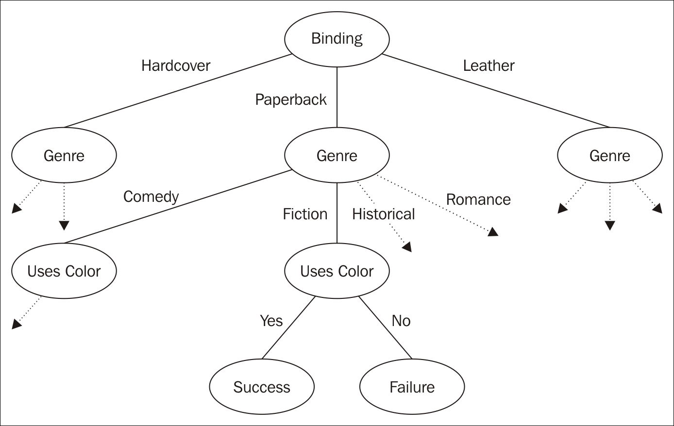
Decision tree
Decision trees are useful and easy to understand. Preparing data for a model is straightforward even for large datasets.
A tree can be taught by dividing an input dataset by the features. This is often done in a recursive fashion and is called recursive partitioning or Top-Down Induction of Decision Trees (TDIDT). The recursion is bounded when node's values are all of the same type as the target or the recursion no longer adds value.
Classification and Regression Tree (CART) analysis refers to two different types of decision tree types:
- Classification tree analysis: The leaf corresponds to a target feature
- Regression tree analysis: The leaf possesses a real number representing a feature
During the process of analysis, multiple trees may be created. There are several techniques used to create trees. The techniques are called ensemble methods:
- Bagging decision trees: The data is resampled and frequently used to obtain a prediction based on consensus
- Random forest classifier: Used to improve the classification rate
- Boosted trees: This can be used for regression or classification problems
- Rotation forest: Uses a technique called Principal Component Analysis (PCA)
With a given set of data, it is possible that more than one tree models the data. For example, the root of a tree may specify whether a bank has an ATM machine and a subsequent internal node may specify the number of tellers. However, the tree could be created where the number of tellers is at the root and the existence of an ATM is an internal node. The difference in the structure of the tree can determine how efficient the tree is.
There are a number of ways of determining the order of the nodes of a tree. One technique is to select an attribute that provides the most information gain; that is, choose an attribute that better helps narrow down the possible decisions fastest.
There are several Java libraries that support decision trees:
- Weka: http://www.cs.waikato.ac.nz/ml/weka/
- Apache Spark: https://spark.apache.org/docs/1.2.0/mllib-decision-tree.html
- JBoost: http://jboost.sourceforge.net
- MAchine Learning for LanguagE Toolkit (MALLET): http://mallet.cs.umass.edu
We will use Waikato Environment for Knowledge Analysis (Weka) to demonstrate how to create a decision tree in Java. Weka is a tool that has a GUI interface that permits analysis of data. It can also be invoked from the command line or through a Java API, which we will use.
As a tree is being built, a variable is selected to split the tree. There are several techniques used to select a variable. The one we use is determined by how much information is gained by choosing a variable. Specifically, we will use the C4.5 algorithm as supported by Weka's J48 class.
Weka uses an .arff file to hold a dataset. This file is human readable and consists of two sections. The first is a header section; it describes the data in the file. This section uses the ampersand to specify the relation and attributes of the data. The second section is the data section; it consists of a comma-delimited set of data.
For this example, we will use a file called books.arff. It is shown next and uses four features called attributes. The features specify how a book is bound, whether it uses multiple colors, its genre, and a result indicating whether the book was purchased or not. The header section is shown here:
@RELATION book_purchases
@ATTRIBUTE Binding {Hardcover, Paperback, Leather}
@ATTRIBUTE Multicolor {yes, no}
@ATTRIBUTE Genre {fiction, comedy, romance, historical}
@ATTRIBUTE Result {Success, Failure}The data section follows and consists of 13 book entries:
@DATA Hardcover,yes,fiction,Success Hardcover,no,comedy,Failure Hardcover,yes,comedy,Success Leather,no,comedy,Success Leather,yes,historical,Success Paperback,yes,fiction,Failure Paperback,yes,romance,Failure Leather,yes,comedy,Failure Paperback,no,fiction,Failure Paperback,yes,historical,Failure Hardcover,yes,historical,Success Paperback,yes,comedy,Success Hardcover,yes,comedy,Success
We will use the BookDecisionTree class as defined next to process this file. It uses one constructor and three methods:
BookDecisionTree: Reads in the trainer data and creates anInstanceobject used to process the datamain: Drives the applicationperformTraining: Trains the model using the datasetgetTestInstance: Creates a test case
The Instances class holds elements representing the individual dataset elements:
public class BookDecisionTree {
private Instances trainingData;
public static void main(String[] args) {
...
}
public BookDecisionTree(String fileName) {
...
}
private J48 performTraining() {
...
}
private Instance getTestInstance(
...
}
}
The constructor opens a file and uses the BufferReader instance to create an instance of the Instances class. Each element of the dataset will be either a feature or a result. The setClassIndex method specifies the index of the result class. In this case, it is the last index of the dataset and corresponds to success or failure:
public BookDecisionTree(String fileName) {
try {
BufferedReader reader = new BufferedReader(
new FileReader(fileName));
trainingData = new Instances(reader);
trainingData.setClassIndex(
trainingData.numAttributes() - 1);
} catch (IOException ex) {
// Handle exceptions
}
}
We will use the J48 class to generate a decision tree. This class uses the C4.5 decision tree algorithm for generating a pruned or unpruned tree. The setOptions method specifies that an unpruned tree be used. The buildClassifier method actually creates the classifier based on the dataset used:
private J48 performTraining() {
J48 j48 = new J48();
String[] options = {"-U"};
try {
j48.setOptions(options);
j48.buildClassifier(trainingData);
} catch (Exception ex) {
ex.printStackTrace();
}
return j48;
}
We will want to test the model, so we will create an object that implements the Instance interface for each test case. A getTestInstance helper method is passed three arguments representing the three features of a data element. The DenseInstance class is a class that implements the Instance interface. The values passed are assigned to the instance and the instance is returned:
private Instance getTestInstance(
String binding, String multicolor, String genre) {
Instance instance = new DenseInstance(3);
instance.setDataset(trainingData);
instance.setValue(trainingData.attribute(0), binding);
instance.setValue(trainingData.attribute(1), multicolor);
instance.setValue(trainingData.attribute(2), genre);
return instance;
}The main method uses all the previous methods to process and test our book dataset. First, a BookDecisionTree instance is created using the name of the book dataset file:
public static void main(String[] args) {
try {
BookDecisionTree decisionTree =
new BookDecisionTree("books.arff");
...
} catch (Exception ex) {
// Handle exceptions
}
}
Next, the performTraining method is invoked to train the model. We also display the tree:
J48 tree = decisionTree.performTraining(); System.out.println(tree.toString());
When executed, the following will be displayed:
J48 unpruned tree ------------------ Binding = Hardcover: Success (5.0/1.0) Binding = Paperback: Failure (5.0/1.0) Binding = Leather: Success (3.0/1.0) Number of Leaves : 3 Size of the tree : 4
We will test the model with two different test cases. Both use identical code to set up the instance. We use the getTestInstance method with test-case-specific values and then use the instance with classifyInstance to get results. To get something that is more readable, we generate a string, which is then displayed:
Instance testInstance = decisionTree.
getTestInstance("Leather", "yes", "historical");
int result = (int) tree.classifyInstance(testInstance);
String results = decisionTree.trainingData.attribute(3).value(result);
System.out.println(
"Test with: " + testInstance + " Result: " + results);
testInstance = decisionTree.
getTestInstance("Paperback", "no", "historical");
result = (int) tree.classifyInstance(testInstance);
results = decisionTree.trainingData.attribute(3).value(result);
System.out.println(
"Test with: " + testInstance + " Result: " + results);
The result of executing this code is as follows:
Test with: Leather,yes,historical Result: Success Test with: Paperback,no,historical Result: Failure
This matches our expectations. This technique is based on the amount of information gain before and after an ordering decision has been made. This can be measured based on the entropy as calculated here:
Entropy = -portionPos * log2(portionPos) - portionNeg* log2(portionNeg)
In this example, portionPos is the portion of the data that is positive and portionNeg is the portion of the data that is negative. Based on the books file, we can calculate the entropy for the binding as shown in the following table. The information gain is calculated by subtracting the entropy for binding from 1.0:
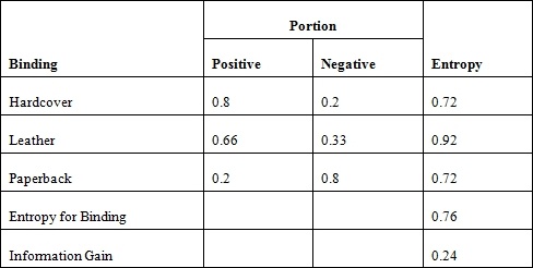
We can calculate the entropy for the use of color and genre in a similar manner. The information gain for color is 0.05, and it is 0.15 for the genre. Thus, it makes more sense to use the binding type for the first level of the tree.
The resulting tree from the example consists of two levels, because the C4.5 algorithm determines that the remaining features do not provide any additional information gain.
Information gain can be problematic when a feature that has a large number of values is chosen, such as a customer's credit card number. Using this type of attribute will quickly narrow down the field, but it is too selective to be of much value.
A Support Vector Machine (SVM) is a supervised machine learning algorithm used for both classification and regression problems. It is mostly used for classification problems. The approach creates a hyperplane to categorize the training data. A hyperplane can be envisioned as a geometric plane that separates two regions. In a two-dimensional space, it will be a line. In a three-dimensional space, it will be a two-dimensional plane. For higher dimensions, it is harder to conceptualize, but they do exist.
Consider the following figure depicting a distribution of two types of data points. The lines represent possible hyperplanes that separate these points. Part of the SVM process is to find the best hyperplane for the problem dataset. We will elaborate on this figure in the coding example.
Hyperplane example
Support vectors are data points that lie near the hyperplane. An SVM model uses the concept of a kernel to map input data to a higher order dimensional space to make the data more easily structured. A mapping function for doing this could lead to an infinite-dimensional space; that is, there could be an unbounded number of possible mappings.
However, what is known as the kernel trick, a kernel function is an approach that avoids this mapping and avoids possibly infeasible computations that might otherwise occur. SVMs support different types of kernels. A list of kernels can be found at http://crsouza.com/2010/03/kernel-functions-for-machine-learning-applications/. Choosing the right kernel depends on the problem. Commonly used kernels include:
- Linear: Uses a linear hyperplane
- Polynomial: Uses a polynomial equation for the hyperplane
- Radial Basis Function (RBF): Uses a non-linear hyperplane
- Sigmoid: The sigmoid kernel, also known as the Hyperbolic Tangent kernel, comes from the neural networks field and is equivalent to a two-layer perceptron neural network
These kernels support different algorithms for analyzing data.
SVMs are useful for higher dimensional spaces that humans have a harder time visualizing. In the previous figure, two attributes were used to predict a third. An SVM can be used when many more attributes are present. The SVM needs to be trained and this can take longer with larger datasets.
We will use the Weka class SMO to demonstrate SVM analysis. The class supports John Platt's sequential minimal optimization algorithm. More information about this algorithm is found at https://www.microsoft.com/en-us/research/publication/fast-training-of-support-vector-machines-using-sequential-minimal-optimization/.
The SMO class supports the following kernels, which can be specified when using the class:
- Puk: The Pearson VII-function-based universal kernel
- PolyKernel: The polynomial kernel
- RBFKernel: The RBF kernel
The algorithm uses training data to create a classification model. Test data can then be used to evaluate the model. We can also evaluate individual data elements.
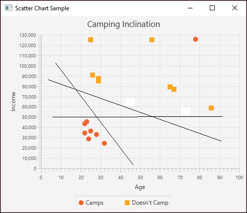
For illustration purposes, we will be using a dataset consisting of age, income, and whether someone camps. We would like to be able to predict whether someone is inclined to camp based on their age and income. The data we use is stored in .arff format and is not based on a survey but has been created to explain the SVM process. The input data is found in the camping.txt file, as shown next. The file extension does not need to be .arff:
@relation camping
@attribute age numeric
@attribute income numeric
@attribute camps {1, 0}
@data
23,45600,1
45,65700,1
72,55600,1
24,28700,1
22,34200,1
28,32800,1
32,24600,1
25,36500,1
26,91000,0
29,85300,0
67,76800,0
86,58900,0
56,125300,0
25,125000,0
22,43600,1
78,125700,1
73,56500,1
29,87600,0
65,79300,0The following shows how the data is distributed graphically. Notice the outlier found in the upper-right corner. The JavaFX code that produces this graph is found at http://www.packtpub.com/support:
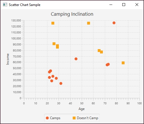
Camping Graph
We will start by reading in the data and handling exceptions:
try {
BufferedReader datafile;
datafile = readDataFile("camping.txt");
...
} catch (Exception ex) {
// Handle exceptions
}
The readDataFile method follows:
public BufferedReader readDataFile(String filename) {
BufferedReader inputReader = null;
try {
inputReader = new BufferedReader(
new FileReader(filename));
} catch (FileNotFoundException ex) {
// Handle exceptions
}
return inputReader;
}The Instances class holds a series of data instances, where each instance is an age, income, and camping value. The setClassIndex method indicates which of the attributes is to be predicted. In this case, it is the camps attribute:
Instances data = new Instances(datafile);
data.setClassIndex(data.numAttributes() - 1);
To train the model, we will split the dataset into two sets. The first 14 instances are used to train the model and the last 5 instances are used to test the model. The second argument of the Instances constructor specifies the beginning index in the dataset, and the last argument specifies how many instances to include:
Instances trainingData = new Instances(data, 0, 14);
Instances testingData = new Instances(data, 14, 5);
An Evaluation class instance is created to evaluate the model. An instance of the SMO class is also created. The SMO class's buildClassifier method builds the classifier using the dataset:
Evaluation evaluation = new Evaluation(trainingData);
Classifier smo = new SMO();
smo.buildClassifier(data);
The evaluateModel method evaluates the model using the testing data. The results are then displayed:
evaluation.evaluateModel(smo, testingData);
System.out.println(evaluation.toSummaryString());
The output follows. Notice one incorrectly classified instance. This corresponds to the outlier mentioned earlier:
Correctly Classified Instances 4 80 % Incorrectly Classified Instances 1 20 % Kappa statistic 0.6154 Mean absolute error 0.2 Root mean squared error 0.4472 Relative absolute error 41.0256 % Root relative squared error 91.0208 % Coverage of cases (0.95 level) 80 % Mean rel. region size (0.95 level) 50 % Total Number of Instances 5
We can also test an individual instance using the classifyInstance method. In the following sequence, we create a new instance using the DenseInstance class. It is then populated using the attributes of the camping dataset:
Instance instance = new DenseInstance(3);
instance.setValue(data.attribute("age"), 78);
instance.setValue(data.attribute("income"), 125700);
instance.setValue(data.attribute("camps"), 1);
The instance needs to be associated with the dataset using the setDataset method:
instance.setDataset(data);
The classifyInstance method is then applied to the smo instance and the results are displayed:
System.out.println(smo.classifyInstance(instance));
When executed, we get the following output:
1.0
There are also alternate testing approaches. A common one is called cross-validation folds. This approach divides the dataset into folds, which are partitions of the dataset. Frequently, 10 partitions are created. Nine of the partitions are used for training and one for testing. This is repeated 10 times using a different partition of the dataset each time, and the average of the results is used. This technique is described at https://weka.wikispaces.com/Generating+cross-validation+folds+(Java+approach).
We will now examine the purpose and use of Bayesian networks.
Bayesian networks, also known as Bayes nets or belief networks, are models designed to reflect a particular world or environment by depicting the states of different attributes of the world and their statistical relationships. The models can be used to show a wide variety of real-world scenarios. In the following diagram, we model a system depicting the relationship between various factors and our likelihood of being late to work:
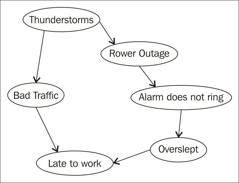
Bayesian network
Each circle on the diagram represents a node or part of the system, which can have various values and probabilities for each value. For example, Power Outage might be true or false — either the power went out or it did not. The probability of the power going out affects the probability that your alarm will not ring, you might oversleep, and thus be late to work.
The nodes at the top of the diagram tend to imply a higher level of causality than those at the bottom. The higher nodes are called parent nodes, and they may have one or more child nodes. Bayesian networks only relate nodes that have a causal dependency and therefore allow more efficient computation of probabilities. Unlike other models, we would not have to store and analyze every possible combination of states of each node. Instead, we can calculate and store probabilities of related nodes. Additionally, Bayesian networks are easily adaptable and can grow as more knowledge about a particular world is acquired.
To model this type of network using Java, we will create a network using JBayes (https://github.com/vangj/jbayes). JBayes is an open source library for creating a simple Bayesian Belief Network (BBN). It is available at no cost for personal or commercial use. In our next example, we will perform approximate inference, a technique considered less accurate but allowing for decreased computational time. This technique is often used when working with big data because it produces a reliable model in a reasonable amount of time. We conduct approximate inference by using weight sampling of each node. JBayes also provides support for exact inference. Exact inference is most often used with smaller datasets or in situations where accuracy is of most importance. JBayes performs exact inference using the junction tree algorithm.
To begin our approximate inference model, we will first create our nodes. We will use the preceding diagram depicting attributes affecting on-time arrival to work to build our network. In the following code example, we use method chaining to create our nodes. Three of the methods take a String parameter. The name method is the name associated with each node. For brevity, we are only using the first initial, so s represents storms, t represents traffic, and so on. The value method allows us to set values for the node. In each case, our nodes can only have two values: t for true or f for false:
Node storms = Node.newBuilder().name("s").value("t").value("f").build();
Node traffic = Node.newBuilder().name("t").value("t").value("f").build();
Node powerOut = Node.newBuilder().name("p").value("t").value("f").build();
Node alarm = Node.newBuilder().name("a").value("t").value("f").build();
Node overslept = Node.newBuilder().name("o").value("t").value("f").build();
Node lateToWork = Node.newBuilder().name("l").value("t").value("f").build();
Next, we assign parents to each of our child nodes. Notice that storms is a parent node to both traffic and powerOut. The lateToWork node has two parent nodes, traffic and overslept:
traffic.addParent(storms); powerOut.addParent(storms); lateToWork.addParent(traffic); alarm.addParent(powerOut); overslept.addParent(alarm); lateToWork.addParent(overslept);
Then we define the conditional probability tables (CPTs) for each of our nodes. These tables are basically two-dimensional arrays representing the probabilities of each attribute of each node. If we have more than one parent node, as in the case of the lateToWork node, we need a row for each. We have used arbitrary values for our probabilities in this example, but note that each row must sum to 1.0:
storms.setCpt(new double[][] {{0.7, 0.3}});
traffic.setCpt(new double[][] {{0.8, 0.2}});
powerOut.setCpt(new double[][] {{0.5, 0.5}});
alarm.setCpt(new double[][] {{0.7, 0.3}});
overslept.setCpt(new double[][] {{0.5, 0.5}});
lateToWork.setCpt(new double[][] {
{0.5, 0.5},
{0.5, 0.5}
});
Finally, we create a Graph object and add each node to our graph structure. We then use this graph to perform our sampling:
Graph bayesGraph = new Graph(); bayesGraph.addNode(storms); bayesGraph.addNode(traffic); bayesGraph.addNode(powerOut); bayesGraph.addNode(alarm); bayesGraph.addNode(overslept); bayesGraph.addNode(lateToWork); bayesGraph.sample(1000);
At this point, we may be interested in the probabilities of each event. We can use the prob method to check the probabilities of a True or False value for each node:
double[] stormProb = storms.probs();
double[] trafProb = traffic.probs();
double[] powerProb = powerOut.probs();
double[] alarmProb = alarm.probs();
double[] overProb = overslept.probs();
double[] lateProb = lateToWork.probs();
out.println("nStorm Probabilities");
out.println("True: " + stormProb[0] + " False: " + stormProb[1]);
out.println("nTraffic Probabilities");
out.println("True: " + trafProb[0] + " False: " + trafProb[1]);
out.println("nPower Outage Probabilities");
out.println("True: " + powerProb[0] + " False: " + powerProb[1]);
out.println("vAlarm Probabilities");
out.println("True: " + alarmProb[0] + " False: " + alarmProb[1]);
out.println("nOverslept Probabilities");
out.println("True: " + overProb[0] + " False: " + overProb[1]);
out.println("nLate to Work Probabilities");
out.println("True: " + lateProb[0] + " False: " + lateProb[1]);
Our output contains the probabilities of each value for each node. For example, the probability of a storm occurring is 71% while the probability of a storm not occurring is 29%:
Storm Probabilities True: 0.71 False: 0.29 Traffic Probabilities True: 0.726 False: 0.274 Power Outage Probabilities True: 0.442 False: 0.558 Alarm Probabilities True: 0.543 False: 0.457 Overslept Probabilities True: 0.556 False: 0.444 Late to Work Probabilities True: 0.469 False: 0.531
Note
Notice in this example that we have used numbers that produce a very high likelihood of being late to work, roughly 47%. This is due to the fact that we have set the probabilities of our parent nodes fairly high as well. This data would vary dramatically if the chances of a storm were lower or if we changed some of the other child nodes as well.
If we would like to save information about our sample, we can save the data to a CSV file using the following code:
try {
CsvUtil.saveSamples(bayesGraph, new FileWriter(
new File("C://JBayesInfo.csv")));
} catch (IOException e) {
// Handle exceptions
}
With this discussion of supervised learning complete, we will now move on to unsupervised learning.
Unsupervised machine learning does not use annotated data; that is, the dataset does to contain anticipated results. While there are several unsupervised learning algorithms, we will demonstrate the use of association rule learning to illustrate this learning approach.
Association rule learning is a technique that identifies relationships between data items. It is part of what is called market basket analysis. When a shopper makes purchases, these purchases are likely to consist of more than one item, and when it does, there are certain items that tend to be bought together. Association rule learning is one approach for identifying these related items. When an association is found, a rule can be formulated for it.
For example, if a customer buys diapers and lotion, they are also likely to buy baby wipes. An analysis can find these associations and a rule stating the observation can be formed. The rule would be expressed as {diapers, lotion} => {wipes}. Being able to identify these purchasing patterns allows a store to offer special coupons, arrange their products to be easier to get, or effect any number of other market-related activities.
One of the problems with this technique is that there are a large number of possible associations. One efficient method that is commonly used is the apriori algorithm. This algorithm works on a collection of transactions defined by a set of items. These items can be thought of as purchases and a transaction as a set of items bought together. The collection is often referred to as a database.
Consider the following set of transactions where a 1 indicates that the item was purchased as part of a transaction and 0 means that it was not purchased:
|
Transaction ID |
Diapers |
Lotion |
Wipes |
Formula |
|
1 |
1 |
1 |
1 |
0 |
|
2 |
1 |
1 |
1 |
1 |
|
3 |
0 |
1 |
1 |
0 |
|
4 |
1 |
0 |
0 |
0 |
|
5 |
0 |
1 |
1 |
1 |
There are several analysis terms used with the apriori model:
- Support: This is the proportion of the items in a database that contain a subset of items. In the previous database, the item {diapers, lotion} occurs 2/5 times or 20%.
- Confidence: This is a measure of the frequency of the rule being true. It is calculated as conf(X- > Y) = sup(X ∪ Y)/sup(X).
- Lift: This measures the degree to which the items are dependent upon each other. It is defined as lift(X -> Y) = sup(X ∪ Y) / (sup(X) * sup(Y)).
- Leverage: Leverage is a measure of the number of transactions that are covered by both X and Y if X and Y are independent of each other. A value above 0 is a good indicator. It is calculated as lev(X->Y) = sup(X ,Y) - sup(X) * sup(Y).
- Conviction: A measure of how often the rule makes an incorrect decision. It is defined as conv(X -> Y) = 1 - sup(Y) / (1 - conf(X -> Y)).
These definitions and sample values can be found at https://en.wikipedia.org/wiki/Association_rule_learning.
We will be using the Apriori Weka class to demonstrate Java support for the algorithm using two datasets. The first is the data discussed previously and the second deals with what a person may take on a hike.
The following is the data file, babies.arff, for baby information:
@relation TEST_ITEM_TRANS
@attribute Diapers {1, 0}
@attribute Lotion {1, 0}
@attribute Wipes {1, 0}
@attribute Formula {1, 0}
@data
1,1,1,0
1,1,1,1
0,1,1,0
1,0,0,0
0,1,1,1We start by reading in the file using a BufferedReader instance. This object is used as the argument of the Instances class, which will hold the data:
try {
BufferedReader br;
br = new BufferedReader(new FileReader("babies.arff"));
Instances data = new Instances(br);
br.close();
...
} catch (Exception ex) {
// Handle exceptions
}
Next, an Apriori instance is created. We set the number of rules to be generated and a minimum confidence for the rules:
Apriori apriori = new Apriori(); apriori.setNumRules(100); apriori.setMinMetric(0.5);
The buildAssociations method generates the associations using the Instances variable. The associations are then displayed:
apriori.buildAssociations(data); System.out.println(apriori);
There will be 100 rules displayed. The following is the abbreviated output. Each rule is followed by various measures of the rule:
Apriori ======= Minimum support: 0.3 (1 instances) Minimum metric <confidence>: 0.5 Number of cycles performed: 14 Generated sets of large itemsets: Size of set of large itemsets L(1): 8 Size of set of large itemsets L(2): 18 Size of set of large itemsets L(3): 16 Size of set of large itemsets L(4): 5 Best rules found: 1. Wipes=1 4 ==> Lotion=1 4 <conf:(1)> lift:(1.25) lev:(0.16) [0] conv:(0.8) 2. Lotion=1 4 ==> Wipes=1 4 <conf:(1)> lift:(1.25) lev:(0.16) [0] conv:(0.8) 3. Diapers=0 2 ==> Lotion=1 2 <conf:(1)> lift:(1.25) lev:(0.08) [0] conv:(0.4) 4. Diapers=0 2 ==> Wipes=1 2 <conf:(1)> lift:(1.25) lev:(0.08) [0] conv:(0.4) 5. Formula=1 2 ==> Lotion=1 2 <conf:(1)> lift:(1.25) lev:(0.08) [0] conv:(0.4) 6. Formula=1 2 ==> Wipes=1 2 <conf:(1)> lift:(1.25) lev:(0.08) [0] conv:(0.4) 7. Diapers=1 Wipes=1 2 ==> Lotion=1 2 <conf:(1)> lift:(1.25) lev:(0.08) [0] conv:(0.4) 8. Diapers=1 Lotion=1 2 ==> Wipes=1 2 <conf:(1)> lift:(1.25) lev:(0.08) [0] conv:(0.4) ... 62. Diapers=0 Lotion=1 Formula=1 1 ==> Wipes=1 1 <conf:(1)> lift:(1.25) lev:(0.04) [0] conv:(0.2) ... 99. Lotion=1 Formula=1 2 ==> Diapers=1 1 <conf:(0.5)> lift:(0.83) lev:(-0.04) [0] conv:(0.4) 100. Diapers=1 Lotion=1 2 ==> Formula=1 1 <conf:(0.5)> lift:(1.25) lev:(0.04) [0] conv:(0.6)
This provides us with a list of relationships, which we can use to identify patterns in activities such as purchasing behavior.
Association rule learning
Association rule learning is a technique that identifies relationships between data items. It is part of what is called market basket analysis. When a shopper makes purchases, these purchases are likely to consist of more than one item, and when it does, there are certain items that tend to be bought together. Association rule learning is one approach for identifying these related items. When an association is found, a rule can be formulated for it.
For example, if a customer buys diapers and lotion, they are also likely to buy baby wipes. An analysis can find these associations and a rule stating the observation can be formed. The rule would be expressed as {diapers, lotion} => {wipes}. Being able to identify these purchasing patterns allows a store to offer special coupons, arrange their products to be easier to get, or effect any number of other market-related activities.
One of the problems with this technique is that there are a large number of possible associations. One efficient method that is commonly used is the apriori algorithm. This algorithm works on a collection of transactions defined by a set of items. These items can be thought of as purchases and a transaction as a set of items bought together. The collection is often referred to as a database.
Consider the following set of transactions where a 1 indicates that the item was purchased as part of a transaction and 0 means that it was not purchased:
|
Transaction ID |
Diapers |
Lotion |
Wipes |
Formula |
|
1 |
1 |
1 |
1 |
0 |
|
2 |
1 |
1 |
1 |
1 |
|
3 |
0 |
1 |
1 |
0 |
|
4 |
1 |
0 |
0 |
0 |
|
5 |
0 |
1 |
1 |
1 |
There are several analysis terms used with the apriori model:
- Support: This is the proportion of the items in a database that contain a subset of items. In the previous database, the item {diapers, lotion} occurs 2/5 times or 20%.
- Confidence: This is a measure of the frequency of the rule being true. It is calculated as conf(X- > Y) = sup(X ∪ Y)/sup(X).
- Lift: This measures the degree to which the items are dependent upon each other. It is defined as lift(X -> Y) = sup(X ∪ Y) / (sup(X) * sup(Y)).
- Leverage: Leverage is a measure of the number of transactions that are covered by both X and Y if X and Y are independent of each other. A value above 0 is a good indicator. It is calculated as lev(X->Y) = sup(X ,Y) - sup(X) * sup(Y).
- Conviction: A measure of how often the rule makes an incorrect decision. It is defined as conv(X -> Y) = 1 - sup(Y) / (1 - conf(X -> Y)).
These definitions and sample values can be found at https://en.wikipedia.org/wiki/Association_rule_learning.
We will be using the Apriori Weka class to demonstrate Java support for the algorithm using two datasets. The first is the data discussed previously and the second deals with what a person may take on a hike.
The following is the data file, babies.arff, for baby information:
@relation TEST_ITEM_TRANS
@attribute Diapers {1, 0}
@attribute Lotion {1, 0}
@attribute Wipes {1, 0}
@attribute Formula {1, 0}
@data
1,1,1,0
1,1,1,1
0,1,1,0
1,0,0,0
0,1,1,1We start by reading in the file using a BufferedReader instance. This object is used as the argument of the Instances class, which will hold the data:
try {
BufferedReader br;
br = new BufferedReader(new FileReader("babies.arff"));
Instances data = new Instances(br);
br.close();
...
} catch (Exception ex) {
// Handle exceptions
}
Next, an Apriori instance is created. We set the number of rules to be generated and a minimum confidence for the rules:
Apriori apriori = new Apriori(); apriori.setNumRules(100); apriori.setMinMetric(0.5);
The buildAssociations method generates the associations using the Instances variable. The associations are then displayed:
apriori.buildAssociations(data); System.out.println(apriori);
There will be 100 rules displayed. The following is the abbreviated output. Each rule is followed by various measures of the rule:
Apriori ======= Minimum support: 0.3 (1 instances) Minimum metric <confidence>: 0.5 Number of cycles performed: 14 Generated sets of large itemsets: Size of set of large itemsets L(1): 8 Size of set of large itemsets L(2): 18 Size of set of large itemsets L(3): 16 Size of set of large itemsets L(4): 5 Best rules found: 1. Wipes=1 4 ==> Lotion=1 4 <conf:(1)> lift:(1.25) lev:(0.16) [0] conv:(0.8) 2. Lotion=1 4 ==> Wipes=1 4 <conf:(1)> lift:(1.25) lev:(0.16) [0] conv:(0.8) 3. Diapers=0 2 ==> Lotion=1 2 <conf:(1)> lift:(1.25) lev:(0.08) [0] conv:(0.4) 4. Diapers=0 2 ==> Wipes=1 2 <conf:(1)> lift:(1.25) lev:(0.08) [0] conv:(0.4) 5. Formula=1 2 ==> Lotion=1 2 <conf:(1)> lift:(1.25) lev:(0.08) [0] conv:(0.4) 6. Formula=1 2 ==> Wipes=1 2 <conf:(1)> lift:(1.25) lev:(0.08) [0] conv:(0.4) 7. Diapers=1 Wipes=1 2 ==> Lotion=1 2 <conf:(1)> lift:(1.25) lev:(0.08) [0] conv:(0.4) 8. Diapers=1 Lotion=1 2 ==> Wipes=1 2 <conf:(1)> lift:(1.25) lev:(0.08) [0] conv:(0.4) ... 62. Diapers=0 Lotion=1 Formula=1 1 ==> Wipes=1 1 <conf:(1)> lift:(1.25) lev:(0.04) [0] conv:(0.2) ... 99. Lotion=1 Formula=1 2 ==> Diapers=1 1 <conf:(0.5)> lift:(0.83) lev:(-0.04) [0] conv:(0.4) 100. Diapers=1 Lotion=1 2 ==> Formula=1 1 <conf:(0.5)> lift:(1.25) lev:(0.04) [0] conv:(0.6)
This provides us with a list of relationships, which we can use to identify patterns in activities such as purchasing behavior.
Using association rule learning to find buying relationships
We will be using the Apriori Weka class to demonstrate Java support for the algorithm using two datasets. The first is the data discussed previously and the second deals with what a person may take on a hike.
The following is the data file, babies.arff, for baby information:
@relation TEST_ITEM_TRANS
@attribute Diapers {1, 0}
@attribute Lotion {1, 0}
@attribute Wipes {1, 0}
@attribute Formula {1, 0}
@data
1,1,1,0
1,1,1,1
0,1,1,0
1,0,0,0
0,1,1,1We start by reading in the file using a BufferedReader instance. This object is used as the argument of the Instances class, which will hold the data:
try {
BufferedReader br;
br = new BufferedReader(new FileReader("babies.arff"));
Instances data = new Instances(br);
br.close();
...
} catch (Exception ex) {
// Handle exceptions
}
Next, an Apriori instance is created. We set the number of rules to be generated and a minimum confidence for the rules:
Apriori apriori = new Apriori(); apriori.setNumRules(100); apriori.setMinMetric(0.5);
The buildAssociations method generates the associations using the Instances variable. The associations are then displayed:
apriori.buildAssociations(data); System.out.println(apriori);
There will be 100 rules displayed. The following is the abbreviated output. Each rule is followed by various measures of the rule:
Apriori ======= Minimum support: 0.3 (1 instances) Minimum metric <confidence>: 0.5 Number of cycles performed: 14 Generated sets of large itemsets: Size of set of large itemsets L(1): 8 Size of set of large itemsets L(2): 18 Size of set of large itemsets L(3): 16 Size of set of large itemsets L(4): 5 Best rules found: 1. Wipes=1 4 ==> Lotion=1 4 <conf:(1)> lift:(1.25) lev:(0.16) [0] conv:(0.8) 2. Lotion=1 4 ==> Wipes=1 4 <conf:(1)> lift:(1.25) lev:(0.16) [0] conv:(0.8) 3. Diapers=0 2 ==> Lotion=1 2 <conf:(1)> lift:(1.25) lev:(0.08) [0] conv:(0.4) 4. Diapers=0 2 ==> Wipes=1 2 <conf:(1)> lift:(1.25) lev:(0.08) [0] conv:(0.4) 5. Formula=1 2 ==> Lotion=1 2 <conf:(1)> lift:(1.25) lev:(0.08) [0] conv:(0.4) 6. Formula=1 2 ==> Wipes=1 2 <conf:(1)> lift:(1.25) lev:(0.08) [0] conv:(0.4) 7. Diapers=1 Wipes=1 2 ==> Lotion=1 2 <conf:(1)> lift:(1.25) lev:(0.08) [0] conv:(0.4) 8. Diapers=1 Lotion=1 2 ==> Wipes=1 2 <conf:(1)> lift:(1.25) lev:(0.08) [0] conv:(0.4) ... 62. Diapers=0 Lotion=1 Formula=1 1 ==> Wipes=1 1 <conf:(1)> lift:(1.25) lev:(0.04) [0] conv:(0.2) ... 99. Lotion=1 Formula=1 2 ==> Diapers=1 1 <conf:(0.5)> lift:(0.83) lev:(-0.04) [0] conv:(0.4) 100. Diapers=1 Lotion=1 2 ==> Formula=1 1 <conf:(0.5)> lift:(1.25) lev:(0.04) [0] conv:(0.6)
This provides us with a list of relationships, which we can use to identify patterns in activities such as purchasing behavior.
Reinforcement learning is a type of learning at the cutting edge of current research into neural networks and machine learning. Unlike unsupervised and supervised learning, reinforcement learning makes decisions based upon the results of an action. It is a goal-oriented learning process, similar to that used by many parents and teachers across the world. We teach children to study and perform well on tests so that they receive high grades as a reward. Likewise, reinforcement learning can be used to teach machines to make choices that will result in the highest reward.
There are four main components to reinforcement learning: the actor or agent, the state or scenario, the chosen action, and the reward. The actor is the object or vehicle making the decisions within the application. The state is the world the actor exists within. Any decision the actor makes occurs within the parameters of the state. The action is simply the choice the actor makes when given a set of options. The reward is the result of each action and influences the likelihood of choosing that particular action in the future.
It is essential to note that the action and the state where the action occurred are not independent. In fact, the correct, or highest rewarding, action can often depend upon the state in which the action occurs. If the actor is trying to decide how to cross a body of water, swimming might be a good option if the body of water is calm and rather small. Swimming would be a terrible choice for the actor to choose if he wanted to cross the Pacific Ocean.
To handle this problem, we can consider the Q function. This function results from the mapping of a particular state to an action within the state. The Q function would link a lower reward to swimming across the Pacific that it might for swimming across a small river. Rather than saying swimming is a low reward activity, the Q function allows for swimming to sometimes have a low reward and other times a higher reward.
Reinforcement learning always begins with a blank slate. The actor does not know the best path or sequence of decisions when the iteration first begins. However, after many iterations through a given problem, considering the results of each particular state-action pair choice, the algorithm improves and learns to make the highest rewarding choices.
The algorithms used to achieve reinforcement learning involve maximization of reward amidst a complex set of processes and choices. Though currently being tested in video games and other discrete environments, the ultimate goal is success of these algorithms in unpredictable, real-world scenarios. Within the topic of reinforcement learning, there are three main flavors or types: temporal difference learning, Q`-learning, and State-Action-Reward-State-Action (SARSA).
Temporal difference learning takes into account previously learned information to inform future decisions. This type of learning assumes a correlation between past and future decisions. Before an action is taken, a prediction is made. This prediction is compared to other known information about the environment and similar decisions before an action is chosen. This process is known as bootstrapping and is thought to create more accurate and useful results.
Q-learning uses the Q function mentioned above to select not only the best action for one particular step in a given state, but the action that will lead to the highest reward from that point forward. This is known as the optimum policy. One great advantage Q-learning offers is the ability to make decisions without requiring a full model of the state. This allows it to function in states with random changes in actions and rewards.
SARSA is another algorithm used in reinforcement learning. Its name is fairly self-explanatory: the Q value depends upon the current State, the current chosen Action, the Reward for that action, the State the agent will exist in after the action is completed, and the subsequent Action taken in the new state. This algorithm looks further ahead one step to make the best possible decision.
There are limited tools currently available for performing reinforcement learning using Java. One popular tool is Platform for Implementing Q-Learning Experiments (Piqle). This Java framework aims to provide tools for fast designing and testing or reinforcement learning experiments. Piqle can be downloaded from http://piqle.sourceforge.net. Another robust tool is called Brown-UMBC Reinforcement Learning and Planning (BURPLAP). Found at http://burlap.cs.brown.edu, this library is also designed for development of algorithms and domains for reinforcement learning. This particular resource boasts in the flexibility of states and actions and supports a wide range of planning and learning algorithms. BURLAP also includes analysis tools for visualization purposes.
Machine learning is concerned with developing techniques that allow the applications to learn without having to be explicitly programmed to solve a problem. This flexibility allows such applications to be used in more varied settings with little to no modifications.
We saw how training data is used to create a model. Once the model has been trained, the model is evaluated using testing data. Both the training data and testing data come from the problem domain. Once trained, the model is used with other input data to make predictions.
We learned how the Weka Java API is used to create decision trees. This tree consists of internal nodes that represent different attributes of the problem. The leaves of the tree represent results. Since there are many ways of constructing a tree, part of the job of a decision tree is to create the best tree.
Support vector machines divide a dataset into sections thus classifying elements in the dataset. This classification s based on the attributes of the data such as age, hair color, or weight. With the model, it is possible to predict outcomes based on attributes of a data instance.
Bayesian networks are used to make predictions based on parent-child relationships between nodes. The probability of one event directly affects the probability of a child event, and we can use this information to predict outcomes of complex real-world environments.
In the section on association rule learning, we learned how the relationships between elements of a dataset can be identified. The more significant relationships allow us to create rules that are applied to solve various problems.
In our discussion of reinforcement learning, we discussed the elements of agent, state, action, and reward and their relationship to one another. We also discussed specific types of reinforcement learning and provided resources for further inquiry.
Having introduced the elements of machine learning, we are now ready to explore neural networks, found in the next chapter.