

The use of sound, images, and videos is becoming a more important aspect of our day-to-day lives. Phone conversations and devices reliant on voice commands are increasingly common. People regularly conduct video chats with other people around the world. There has been a rapid proliferation of photo and video sharing sites. Applications that utilize images, video, and sound from a variety of sources are becoming more common.
In this chapter, we will demonstrate several techniques available to Java to process sounds and images. The first part of the chapter addresses sound processing. Both speech recognition and Text-To-Speech (TTS) APIs will be demonstrated. Specifically, we will use the FreeTTS (http://freetts.sourceforge.net/docs/index.php) API to convert text to speech, followed with a demonstration of the CMU Sphinx toolkit for speech recognition.
The Java Speech API (JSAPI) (http://www.oracle.com/technetwork/java/index-140170.html) provides access to speech technology. It is not part of the standard JDK but is supported by third-party vendors. Its intent is to support speech recognition and speech synthesizers. There are several vendors that support JSAPI, including FreeTTS and Festival (http://www.cstr.ed.ac.uk/projects/festival/).
In addition, there are several cloud-based speech APIs, including IBM's support through Watson Cloud speech-to-text capabilities.
Next, we will examine image processing techniques, including facial recognition. This involves identifying faces within an image. This technique is easy to accomplish using OpenCV (http://opencv.org/) which we will demonstrate in the Identifying faces section.
We will end the chapter with a discussion of Neuroph Studio, a neural network Java-based editor, to classify images and perform image recognition. We will continue to use faces here and attempt to train a network to recognize images of human faces.
Speech synthesis generates human speech. TTS converts text to speech and is useful for a number of different applications. It is used in many places, including phone help desk systems and ordering systems. The TTS process typically consists of two parts. The first part tokenizes and otherwise processes the text into speech units. The second part converts these units into speech.
The two primary approaches for TTS uses concatenation synthesis and formant synthesis. Concatenation synthesis frequently combines prerecorded human speech to create the desired output. Formant synthesis does not use human speech but generates speech by creating electronic waveforms.
We will be using FreeTTS (http://freetts.sourceforge.net/docs/index.php) to demonstrate TTS. The latest version can be downloaded from https://sourceforge.net/projects/freetts/files/. This approach uses concatenation to generate speech.
There are several important terms used in TTS/FreeTTS:
- Utterance - This concept corresponds roughly to the vocal sounds that make up a word or phrase
- Items - Sets of features (name/value pairs) that represent parts of an utterance
- Relationship - A list of items, used by FreeTTS to iterate back and forward through an utterance
- Phone - A distinct sound
- Diphone - A pair of adjacent phones
The FreeTTS Programmer's Guide (http://freetts.sourceforge.net/docs/ProgrammerGuide.html) details the process of converting text to speech. This is a multi-step process whose major steps include the following:
- Tokenization - Extracting the tokens from the text
- TokenToWords - Converting certain words, such as 1910 to nineteen ten
- PartOfSpeechTagger - This step currently does nothing, but is intended to identify the parts of speech
- Phraser - Creates a phrase relationship for the utterance
- Segmenter - Determines where syllable breaks occur
- PauseGenerator - This step inserts pauses within speech, such as before utterances
- Intonator - Determines the accents and tones
- PostLexicalAnalyzer - This step fixes problems such as a mismatch between the available diphones and the one that needs to be spoken
- Durator - Determines the duration of the syllables
- ContourGenerator - Calculates the fundamental frequency curve for an utterance, which maps the frequency against time and contributes to the generation of tones
- UnitSelector - Groups related diphones into a unit
- PitchMarkGenerator - Determines the pitches for an utterance
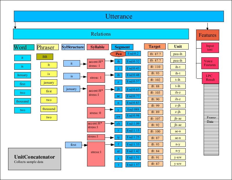
- UnitConcatenator - Concatenates the diphone data together
The following figure is from the FreeTTS Programmer's Guide, Figure 11: The Utterance after UnitConcatenator processing, and depicts the process. This high-level overview of the TTS process provides a hint at the complexity of the process:
TTS system facilitates the use of different voices. For example, these differences may be in the language, the sex of the speaker, or the age of the speaker.
The MBROLA Project's (http://tcts.fpms.ac.be/synthesis/mbrola.html) objective is to support voice synthesizers for as many languages as possible. MBROLA is a speech synthesizer that can be used with a TTS system such as FreeTTS to support TTS synthesis.
Download MBROLA for the appropriate platform binary from http://tcts.fpms.ac.be/synthesis/mbrola.html. From the same page, download any desired MBROLA voices found at the bottom of the page. For our examples we will use usa1, usa2, and usa3. Further details about the setup are found at http://freetts.sourceforge.net/mbrola/README.html.
The following statement illustrates the code needed to access the MBROLA voices. The setProperty method assigns the path where the MBROLA resources are found:
System.setProperty("mbrola.base", "path-to-mbrola-directory");
To demonstrate how to use TTS, we use the following statement. We obtain an instance of the VoiceManager class, which will provide access to various voices:
VoiceManager voiceManager = VoiceManager.getInstance();
To use a specific voice the getVoice method is passed the name of the voice and returns an instance of the Voice class. In this example, we used mbrola_us1, which is a US English, young, female voice:
Voice voice = voiceManager.getVoice("mbrola_us1");
Once we have obtained the Voice instance, use the allocate method to load the voice. The speak method is then used to synthesize the words passed to the method as a string, as illustrated here:
voice.allocate();
voice.speak("Hello World");
When executed, the words "Hello World" should be heard. Try this with other voices, as described in the next section, and text to see which combination is best suited for an application.
The VoiceManager class' getVoices method is used to obtain an array of the voices currently available. This can be useful to provide users with a list of voices to choose from. We will use the method here to illustrate some of the voices available. In the next code sequence, the method returns the array, whose elements are then displayed:
Voice[] voices = voiceManager.getVoices();
for (Voice v : voices) {
out.println(v);
}
The output will be similar to the following:
CMUClusterUnitVoice CMUDiphoneVoice CMUDiphoneVoice MbrolaVoice MbrolaVoice MbrolaVoice
The getVoiceInfo method provides potentially more useful information, though it is somewhat verbose:
out.println(voiceManager.getVoiceInfo());
The first part of the output follows; the VoiceDirectory directory is displayed followed by the details of the voice. Notice that the directory name contains the name of the voice. The KevinVoiceDirectory contains two voices: kevin and kevin16:
VoiceDirectory 'com.sun.speech.freetts.en.us.cmu_time_awb.AlanVoiceDirectory' Name: alan Description: default time-domain cluster unit voice Organization: cmu Domain: time Locale: en_US Style: standard Gender: MALE Age: YOUNGER_ADULT Pitch: 100.0 Pitch Range: 12.0 Pitch Shift: 1.0 Rate: 150.0 Volume: 1.0 VoiceDirectory 'com.sun.speech.freetts.en.us.cmu_us_kal.KevinVoiceDirectory' Name: kevin Description: default 8-bit diphone voice Organization: cmu Domain: general Locale: en_US Style: standard Gender: MALE Age: YOUNGER_ADULT Pitch: 100.0 Pitch Range: 11.0 Pitch Shift: 1.0 Rate: 150.0 Volume: 1.0 Name: kevin16 Description: default 16-bit diphone voice Organization: cmu Domain: general Locale: en_US Style: standard Gender: MALE Age: YOUNGER_ADULT Pitch: 100.0 Pitch Range: 11.0 Pitch Shift: 1.0 Rate: 150.0 Volume: 1.0 ... Using voices from a JAR file
Voices can be stored in JAR files. The VoiceDirectory class provides access to voices stored in this manner. The voice directories available to FreeTTs are found in the lib directory and include the following:
cmu_time_awb.jarcmu_us_kal.jar
The name of a voice directory can be obtained from the command prompt:
java -jar fileName.jar
For example, execute the following command:
java -jar cmu_time_awb.jar
It generates the following output:
VoiceDirectory 'com.sun.speech.freetts.en.us.cmu_time_awb.AlanVoiceDirectory' Name: alan Description: default time-domain cluster unit voice Organization: cmu Domain: time Locale: en_US Style: standard Gender: MALE Age: YOUNGER_ADULT Pitch: 100.0 Pitch Range: 12.0 Pitch Shift: 1.0 Rate: 150.0 Volume: 1.0
The Voice class provides a number of methods that permit the extraction or setting of speech characteristics. As we demonstrated earlier, the VoiceManager class' getVoiceInfo method provided information about the voices currently available. However, we can use the Voice class to get information about a specific voice.
In the following example, we will display information about the voice kevin16. We start by getting an instance of this voice using the getVoice method:
VoiceManager vm = VoiceManager.getInstance();
Voice voice = vm.getVoice("kevin16");
voice.allocate();
Next, we call a number of the Voice class' get method to obtain specific information about the voice. This includes previous information provided by the getVoiceInfo method and other information that is not otherwise available:
out.println("Name: " + voice.getName());
out.println("Description: " + voice.getDescription());
out.println("Organization: " + voice.getOrganization());
out.println("Age: " + voice.getAge());
out.println("Gender: " + voice.getGender());
out.println("Rate: " + voice.getRate());
out.println("Pitch: " + voice.getPitch());
out.println("Style: " + voice.getStyle());
The output of this example follows:
Name: kevin16 Description: default 16-bit diphone voice Organization: cmu Age: YOUNGER_ADULT Gender: MALE Rate: 150.0 Pitch: 100.0 Style: standard
These results are self-explanatory and give you an idea of the type of information available. There are additional methods that give you access to details regarding the TTS process that are not normally of interest. This includes information such as the audio player being used, utterance-specific data, and features of a specific phone.
Having demonstrated how text can be converted to speech, we will now examine how we can convert speech to text.
Converting speech to text is an important application feature. This ability is increasingly being used in a wide variety of contexts. Voice input is used to control smart phones, automatically handle input as part of help desk applications, and to assist people with disabilities, to mention a few examples.
Speech consists of an audio stream that is complex. Sounds can be split into phones, which are sound sequences that are similar. Pairs of these phones are called diphones. Utterances consist of words and various types of pauses between them.
The essence of the conversion process involves splitting sounds by silences between utterances. These utterances are then matched to the words that most closely sound like the utterance. However, this can be difficult due to many factors. For example, these differences may be in the form of variances in how words are pronounced due to the context of the word, regional dialects, the quality of the sound, and other factors.
The matching process is quite involved and often uses multiple models. A model may be used to match acoustic features with a sound. A phonetic model can be used to match phones to words. Another model is used to restrict word searches to a given language. These models are never entirely accurate and contribute to inaccuracies found in the recognition process.
We will be using CMUSphinx 4 to illustrate this process.
Audio processed by CMUSphinx must be in Pulse Code Modulation (PCM) format. PCM is a technique that samples analog data, such as an analog wave representing speech, and produces a digital version of the signal. FFmpeg (https://ffmpeg.org/) is a free tool that can convert between audio formats if needed.
You will need to create sample audio files using the PCM format. These files should be fairly short and can contain numbers or words. It is recommended that you run the examples with different files to see how well the speech recognition works.
First, we set up the basic framework for the conversion by creating a try-catch block to handle exceptions. First, create an instance of the Configuration class. It is used to configure the recognizer to recognize standard English. The configuration models and dictionary need to be changed to handle other languages:
try {
Configuration configuration = new Configuration();
String prefix = "resource:/edu/cmu/sphinx/models/en-us/";
configuration
.setAcousticModelPath(prefix + "en-us");
configuration
.setDictionaryPath(prefix + "cmudict-en-us.dict");
configuration
.setLanguageModelPath(prefix + "en-us.lm.bin");
...
} catch (IOException ex) {
// Handle exceptions
}
The StreamSpeechRecognizer class is then created using configuration. This class processes the speech based on an input stream. In the following code, we create an instance of the StreamSpeechRecognizer class and an InputStream from the speech file:
StreamSpeechRecognizer recognizer = new StreamSpeechRecognizer(
configuration);
InputStream stream = new FileInputStream(new File("filename"));
To start speech processing, the startRecognition method is invoked. The getResult method returns a SpeechResult instance that holds the result of the processing. We then use the SpeechResult method to get the best results. We stop the processing using the stopRecognition method:
recognizer.startRecognition(stream);
SpeechResult result;
while ((result = recognizer.getResult()) != null) {
out.println("Hypothesis: " + result.getHypothesis());
}
recognizer.stopRecognition();
When this is executed, we get the following, assuming the speech file contained this sentence:
Hypothesis: mary had a little lamb
When speech is interpreted there may be more than one possible word sequence. We can obtain the best ones using the getNbest method, whose argument specifies how many possibilities should be returned. The following demonstrates this method:
Collection<String> results = result.getNbest(3);
for (String sentence : results) {
out.println(sentence);
}
One possible output follows:
<s> mary had a little lamb </s> <s> marry had a little lamb </s> <s> mary had a a little lamb </s>
This gives us the basic results. However, we will probably want to do something with the actual words. The technique for getting the words is explained next.
The individual words of the results can be extracted using the getWords method, as shown next. The method returns a list of WordResult instance, each of which represents one word:
List<WordResult> words = result.getWords();
for (WordResult wordResult : words) {
out.print(wordResult.getWord() + " ");
}
The output for this code sequence follows <sil> reflects a silence found at the beginning of the speech:
<sil> mary had a little lamb
We can extract more information about the words using various methods of the WordResult class. In this sequence that follows, we will return the confidence and time frame associated with each word.
The getConfidence method returns the confidence expressed as a log. We use the SpeechResult class' getResult method to get an instance of the Result class. Its getLogMath method is then used to get a LogMath instance. The logToLinear method is passed the confidence value and the value returned is a real number between 0 and 1.0 inclusive. More confidence is reflected by a larger value.
The getTimeFrame method returns a TimeFrame instance. Its toString method returns two integer values, separated by a colon, reflecting the beginning and end times of the word:
for (WordResult wordResult : words) {
out.printf("%s\n\tConfidence: %.3f\n\tTime Frame: %s\n",
wordResult.getWord(), result
.getResult()
.getLogMath()
.logToLinear((float)wordResult
.getConfidence()),
wordResult.getTimeFrame());
}
One possible output follows:
<sil> Confidence: 0.998 Time Frame: 0:430 mary Confidence: 0.998 Time Frame: 440:900 had Confidence: 0.998 Time Frame: 910:1200 a Confidence: 0.998 Time Frame: 1210:1340 little Confidence: 0.998 Time Frame: 1350:1680 lamb Confidence: 0.997 Time Frame: 1690:2170
Now that we have examined how sound can be processed, we will turn our attention to image processing.
Using CMUPhinx to convert speech to text
Audio processed by CMUSphinx must be in Pulse Code Modulation (PCM) format. PCM is a technique that samples analog data, such as an analog wave representing speech, and produces a digital version of the signal. FFmpeg (https://ffmpeg.org/) is a free tool that can convert between audio formats if needed.
You will need to create sample audio files using the PCM format. These files should be fairly short and can contain numbers or words. It is recommended that you run the examples with different files to see how well the speech recognition works.
First, we set up the basic framework for the conversion by creating a try-catch block to handle exceptions. First, create an instance of the Configuration class. It is used to configure the recognizer to recognize standard English. The configuration models and dictionary need to be changed to handle other languages:
try {
Configuration configuration = new Configuration();
String prefix = "resource:/edu/cmu/sphinx/models/en-us/";
configuration
.setAcousticModelPath(prefix + "en-us");
configuration
.setDictionaryPath(prefix + "cmudict-en-us.dict");
configuration
.setLanguageModelPath(prefix + "en-us.lm.bin");
...
} catch (IOException ex) {
// Handle exceptions
}
The StreamSpeechRecognizer class is then created using configuration. This class processes the speech based on an input stream. In the following code, we create an instance of the StreamSpeechRecognizer class and an InputStream from the speech file:
StreamSpeechRecognizer recognizer = new StreamSpeechRecognizer(
configuration);
InputStream stream = new FileInputStream(new File("filename"));
To start speech processing, the startRecognition method is invoked. The getResult method returns a SpeechResult instance that holds the result of the processing. We then use the SpeechResult method to get the best results. We stop the processing using the stopRecognition method:
recognizer.startRecognition(stream);
SpeechResult result;
while ((result = recognizer.getResult()) != null) {
out.println("Hypothesis: " + result.getHypothesis());
}
recognizer.stopRecognition();
When this is executed, we get the following, assuming the speech file contained this sentence:
Hypothesis: mary had a little lamb
When speech is interpreted there may be more than one possible word sequence. We can obtain the best ones using the getNbest method, whose argument specifies how many possibilities should be returned. The following demonstrates this method:
Collection<String> results = result.getNbest(3);
for (String sentence : results) {
out.println(sentence);
}
One possible output follows:
<s> mary had a little lamb </s> <s> marry had a little lamb </s> <s> mary had a a little lamb </s>
This gives us the basic results. However, we will probably want to do something with the actual words. The technique for getting the words is explained next.
The individual words of the results can be extracted using the getWords method, as shown next. The method returns a list of WordResult instance, each of which represents one word:
List<WordResult> words = result.getWords();
for (WordResult wordResult : words) {
out.print(wordResult.getWord() + " ");
}
The output for this code sequence follows <sil> reflects a silence found at the beginning of the speech:
<sil> mary had a little lamb
We can extract more information about the words using various methods of the WordResult class. In this sequence that follows, we will return the confidence and time frame associated with each word.
The getConfidence method returns the confidence expressed as a log. We use the SpeechResult class' getResult method to get an instance of the Result class. Its getLogMath method is then used to get a LogMath instance. The logToLinear method is passed the confidence value and the value returned is a real number between 0 and 1.0 inclusive. More confidence is reflected by a larger value.
The getTimeFrame method returns a TimeFrame instance. Its toString method returns two integer values, separated by a colon, reflecting the beginning and end times of the word:
for (WordResult wordResult : words) {
out.printf("%s\n\tConfidence: %.3f\n\tTime Frame: %s\n",
wordResult.getWord(), result
.getResult()
.getLogMath()
.logToLinear((float)wordResult
.getConfidence()),
wordResult.getTimeFrame());
}
One possible output follows:
<sil> Confidence: 0.998 Time Frame: 0:430 mary Confidence: 0.998 Time Frame: 440:900 had Confidence: 0.998 Time Frame: 910:1200 a Confidence: 0.998 Time Frame: 1210:1340 little Confidence: 0.998 Time Frame: 1350:1680 lamb Confidence: 0.997 Time Frame: 1690:2170
Now that we have examined how sound can be processed, we will turn our attention to image processing.
Obtaining more detail about the words
The individual words of the results can be extracted using the getWords method, as shown next. The method returns a list of WordResult instance, each of which represents one word:
List<WordResult> words = result.getWords();
for (WordResult wordResult : words) {
out.print(wordResult.getWord() + " ");
}
The output for this code sequence follows <sil> reflects a silence found at the beginning of the speech:
<sil> mary had a little lamb
We can extract more information about the words using various methods of the WordResult class. In this sequence that follows, we will return the confidence and time frame associated with each word.
The getConfidence method returns the confidence expressed as a log. We use the SpeechResult class' getResult method to get an instance of the Result class. Its getLogMath method is then used to get a LogMath instance. The logToLinear method is passed the confidence value and the value returned is a real number between 0 and 1.0 inclusive. More confidence is reflected by a larger value.
The getTimeFrame method returns a TimeFrame instance. Its toString method returns two integer values, separated by a colon, reflecting the beginning and end times of the word:
for (WordResult wordResult : words) {
out.printf("%s\n\tConfidence: %.3f\n\tTime Frame: %s\n",
wordResult.getWord(), result
.getResult()
.getLogMath()
.logToLinear((float)wordResult
.getConfidence()),
wordResult.getTimeFrame());
}
One possible output follows:
<sil> Confidence: 0.998 Time Frame: 0:430 mary Confidence: 0.998 Time Frame: 440:900 had Confidence: 0.998 Time Frame: 910:1200 a Confidence: 0.998 Time Frame: 1210:1340 little Confidence: 0.998 Time Frame: 1350:1680 lamb Confidence: 0.997 Time Frame: 1690:2170
Now that we have examined how sound can be processed, we will turn our attention to image processing.
The process of extracting text from an image is called O ptical Character Recognition (OCR). This can be very useful when the text data that needs to be processed is embedded in an image. For example, the information contained in license plates, road signs, and directions can be very useful at times.
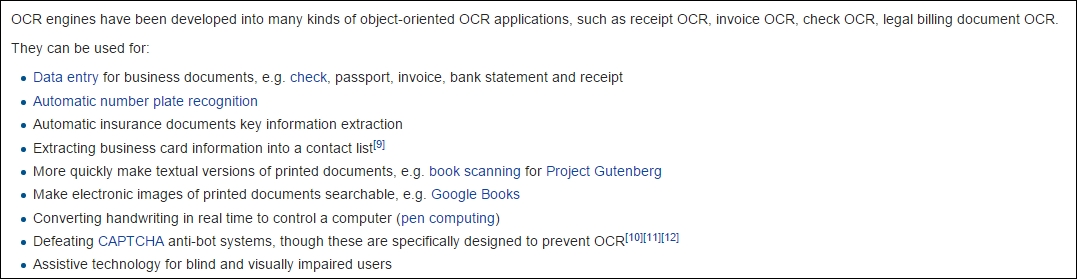
We can perform OCR using Tess4j (http://tess4j.sourceforge.net/), a Java JNA wrapper for Tesseract OCR API. We will demonstrate how to use the API using an image captured from the Wikipedia article on OCR (https://en.wikipedia.org/wiki/Optical_character_recognition#Applications). The Javadoc for the API is found at http://tess4j.sourceforge.net/docs/docs-3.0/. The image we use is shown here:
The ITesseract interface contains numerous OCR methods. The doOCR method takes a file and returns a string containing the words found in the file, as shown here:
ITesseract instance = new Tesseract();
try {
String result = instance.doOCR(new File("OCRExample.png"));
out.println(result);
} catch (TesseractException e) {
// Handle exceptions
}
Part of the output is shown next:
OCR engines nave been developed into many lunds oiobiectorlented OCR applicatlons, sucn as reoeipt OCR, involoe OCR, check OCR, legal billing document OCR They can be used ior - Data entry ior business documents, e g check, passport, involoe, bank statement and receipt - Automatic number plate recognnlon
As you can see, there are numerous errors in this example. Often the quality of an image needs to be improved before it can be processed correctly. Techniques for improving the quality of the output can be found at https://github.com/tesseract-ocr/tesseract/wiki/ImproveQuality. For example, we can use the setLanguage method to specify the language processed. Also, the method often works better on TIFF images.
In the next example, we used an enlarged portion of the previous image, as shown here:
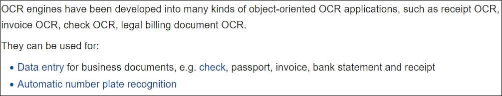
The output is much better, as shown here:
OCR engines have been developed into many kinds of object-oriented OCR applications, such as receipt OCR,
invoice OCR, check OCR, legal billing document OCR.
They can be used for:
. Data entry for business documents, e.g. check, passport, invoice, bank statement and receipt
. Automatic number plate recognition
These examples highlight the need for the careful cleaning of data.
Using Tess4j to extract text
The ITesseract interface contains numerous OCR methods. The doOCR method takes a file and returns a string containing the words found in the file, as shown here:
ITesseract instance = new Tesseract();
try {
String result = instance.doOCR(new File("OCRExample.png"));
out.println(result);
} catch (TesseractException e) {
// Handle exceptions
}
Part of the output is shown next:
OCR engines nave been developed into many lunds oiobiectorlented OCR applicatlons, sucn as reoeipt OCR, involoe OCR, check OCR, legal billing document OCR They can be used ior - Data entry ior business documents, e g check, passport, involoe, bank statement and receipt - Automatic number plate recognnlon
As you can see, there are numerous errors in this example. Often the quality of an image needs to be improved before it can be processed correctly. Techniques for improving the quality of the output can be found at https://github.com/tesseract-ocr/tesseract/wiki/ImproveQuality. For example, we can use the setLanguage method to specify the language processed. Also, the method often works better on TIFF images.
In the next example, we used an enlarged portion of the previous image, as shown here:
The output is much better, as shown here:
OCR engines have been developed into many kinds of object-oriented OCR applications, such as receipt OCR,
invoice OCR, check OCR, legal billing document OCR.
They can be used for:
. Data entry for business documents, e.g. check, passport, invoice, bank statement and receipt
. Automatic number plate recognition
These examples highlight the need for the careful cleaning of data.
Identifying faces within an image is useful in many situations. It can potentially classify an image as one containing people or find people in an image for further processing. We will use OpenCV 3.1 (http://opencv.org/opencv-3-1.html) for our examples.
OpenCV (http://opencv.org/) is an open source computer vision library that supports several programming languages, including Java. It supports a number of techniques, including machine learning algorithms, to perform computer vision tasks. The library supports such operations as face detection, tracking camera movements, extracting 3D models, and removing red eye from images. In this section, we will demonstrate face detection.
The example that follows was adapted from http://docs.opencv.org/trunk/d9/d52/tutorial_java_dev_intro.html. Start by loading the native libraries added to your system when OpenCV was installed. On Windows, this requires that appropriate DLL files are available:
System.loadLibrary(Core.NATIVE_LIBRARY_NAME);
We used a base string to specify the location of needed OpenCV files. Using an absolute path works better with many methods:
String base = "PathToResources";
The CascadeClassifier class is used for object classification. In this case, we will use it for face detection. An XML file is used to initialize the class. In the following code, we use the lbpcascade_frontalface.xml file, which provides information to assist in the identification of objects. In the OpenCV download are several files, as listed here, that can be used for specific face recognition scenarios:
lbpcascade_frontalcatface.xmllbpcascade_frontalface.xmllbpcascade_frontalprofileface.xmllbpcascade_silverware.xml
The following statement initializes the class to detect faces:
CascadeClassifier faceDetector =
new CascadeClassifier(base +
"/lbpcascade_frontalface.xml");
The image to be processed is loaded, as shown here:
Mat image = Imgcodecs.imread(base + "/images.jpg");
For this example, we used the following image:
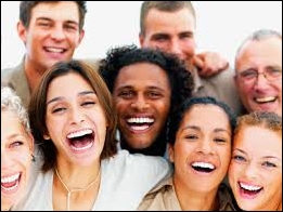
To find this image, perform a Google search using the term people. Select the Images category and then filter for Labeled for reuse. The image has the label: Closeup portrait of a group of business people laughing by Lynda Sanchez.
When faces are detected, the location within the image is stored in a MatOfRect instance. This class is intended to hold vectors and matrixes for any faces found:
MatOfRect faceVectors = new MatOfRect();
At this point, we are ready to detect faces. The detectMultiScale method performs this task. The image and the MatOfRect instance to hold the locations of any images are passed to the method:
faceDetector.detectMultiScale(image, faceVectors);
The next statement shows how many faces were detected:
out.println(faceVectors.toArray().length + " faces found");
We need to use this information to augment the image. This process will draw boxes around each face found, as shown next. To do this, the Imgproc class' rectangle method is used. The method is called once for each face detected. It is passed the image to be modified and the points represented the boundaries of the face:
for (Rect rect : faceVectors.toArray()) {
Imgproc.rectangle(image, new Point(rect.x, rect.y),
new Point(rect.x + rect.width, rect.y + rect.height),
new Scalar(0, 255, 0));
}The last step writes this image to a file using the Imgcodecs class' imwrite method:
Imgcodecs.imwrite("faceDetection.png", image);
As shown in the following image, it was able to identify four images:
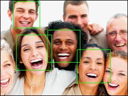
Using different configuration files will work better for other facial profiles.
Using OpenCV to detect faces
The example that follows was adapted from http://docs.opencv.org/trunk/d9/d52/tutorial_java_dev_intro.html. Start by loading the native libraries added to your system when OpenCV was installed. On Windows, this requires that appropriate DLL files are available:
System.loadLibrary(Core.NATIVE_LIBRARY_NAME);
We used a base string to specify the location of needed OpenCV files. Using an absolute path works better with many methods:
String base = "PathToResources";
The CascadeClassifier class is used for object classification. In this case, we will use it for face detection. An XML file is used to initialize the class. In the following code, we use the lbpcascade_frontalface.xml file, which provides information to assist in the identification of objects. In the OpenCV download are several files, as listed here, that can be used for specific face recognition scenarios:
lbpcascade_frontalcatface.xmllbpcascade_frontalface.xmllbpcascade_frontalprofileface.xmllbpcascade_silverware.xml
The following statement initializes the class to detect faces:
CascadeClassifier faceDetector =
new CascadeClassifier(base +
"/lbpcascade_frontalface.xml");
The image to be processed is loaded, as shown here:
Mat image = Imgcodecs.imread(base + "/images.jpg");
For this example, we used the following image:
To find this image, perform a Google search using the term people. Select the Images category and then filter for Labeled for reuse. The image has the label: Closeup portrait of a group of business people laughing by Lynda Sanchez.
When faces are detected, the location within the image is stored in a MatOfRect instance. This class is intended to hold vectors and matrixes for any faces found:
MatOfRect faceVectors = new MatOfRect();
At this point, we are ready to detect faces. The detectMultiScale method performs this task. The image and the MatOfRect instance to hold the locations of any images are passed to the method:
faceDetector.detectMultiScale(image, faceVectors);
The next statement shows how many faces were detected:
out.println(faceVectors.toArray().length + " faces found");
We need to use this information to augment the image. This process will draw boxes around each face found, as shown next. To do this, the Imgproc class' rectangle method is used. The method is called once for each face detected. It is passed the image to be modified and the points represented the boundaries of the face:
for (Rect rect : faceVectors.toArray()) {
Imgproc.rectangle(image, new Point(rect.x, rect.y),
new Point(rect.x + rect.width, rect.y + rect.height),
new Scalar(0, 255, 0));
}The last step writes this image to a file using the Imgcodecs class' imwrite method:
Imgcodecs.imwrite("faceDetection.png", image);
As shown in the following image, it was able to identify four images:
Using different configuration files will work better for other facial profiles.
In this section, we will demonstrate one technique for classifying visual data. We will use Neuroph to accomplish this. Neuroph is a Java-based neural network framework that supports a variety of neural network architectures. Its open source library provides support and plugins for other applications. In this example, we will use its neural network editor, Neuroph Studio, to create a network. This network can be saved and used in other applications. Neuroph Studio is available for download here: http://neuroph.sourceforge.net/download.html. We are building upon the process shown here: http://neuroph.sourceforge.net/image_recognition.htm.
For our example, we will create a Multi Layer Perceptron (MLP) network. We will then train our network to recognize images. We can both train and test our network using Neuroph Studio. It is important to understand how MLP networks recognize and interpret image data. Every image is basically represented by three two-dimensional arrays. Each array contains information about the color components: one array contains information about the color red, one about the color green, and one about the color blue. Every element of the array holds information about one specific pixel in the image. These arrays are then flattened into a one-dimensional array to be used as an input by the neural network.
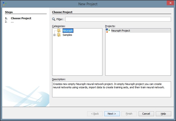
To begin, first create a new Neuroph Studio project:
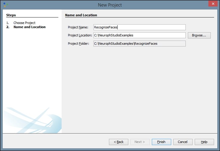
We will name our project RecognizeFaces because we are going train the neural network to recognize images of human faces:
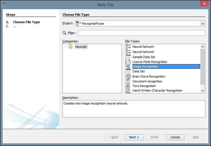
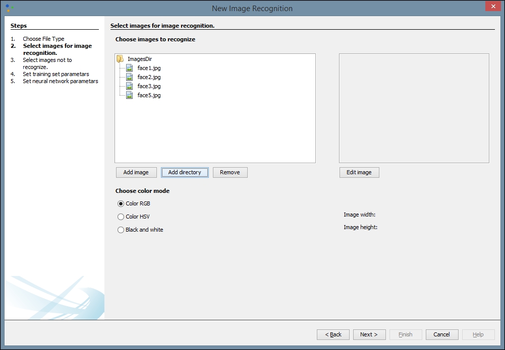
Next, we create a new file in our project. There are many types of project to choose from, but we will choose an Image Recognition type:
Click Next and then click Add directory. We have created a directory on our local machine and added several different black and white images of faces to use for training. These can be found by searching Google images or another search engine. The more quality images you have to train with, theoretically, the better your network will be:
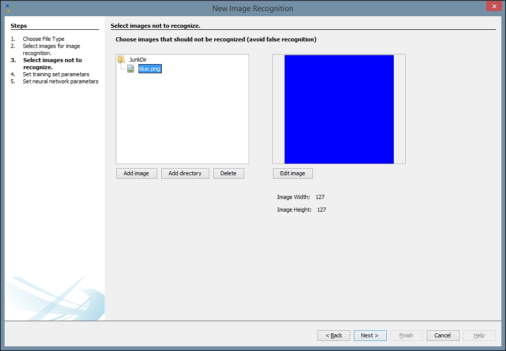
After you click Next, you will be directed to select an image to not recognize. You may need to try different images based upon the images you want to recognize. The image you select here will prevent false recognitions. We have chosen a simple blue square from another directory on our local machine, but if you are using other types of image for training, other color blocks may work better:
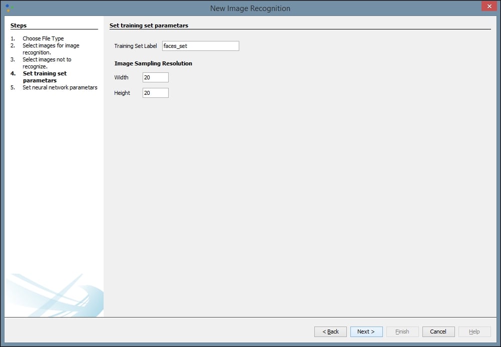
Next, we need to provide network training parameters. We also need to label our training dataset and set our resolution. A height and width of 20 is a good place to start, but you may want to change these values to improve your results. Some trial and error may be involved. The purpose of providing this information is to allow for image scaling. When we scale images to a smaller size, our network can process them and learn faster:
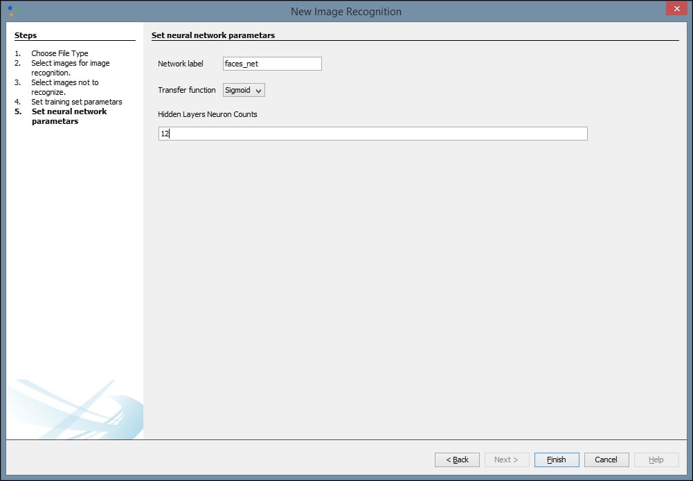
Finally, we can create our network. We assign a label to our network and define our Transfer function. The default function, Sigmoid, will work for most networks, but if your results are not optimal you may want to try Tanh. The default number of Hidden Layers Neuron Counts is 12, and that is a good place to start. Be aware that increasing the number of neurons increases the time it takes to train the network and decreases your ability to generalize the network to other images. As with some of our previous values, some trial and error may be necessary to find the optimal settings for a given network. Select Finish when you are done:
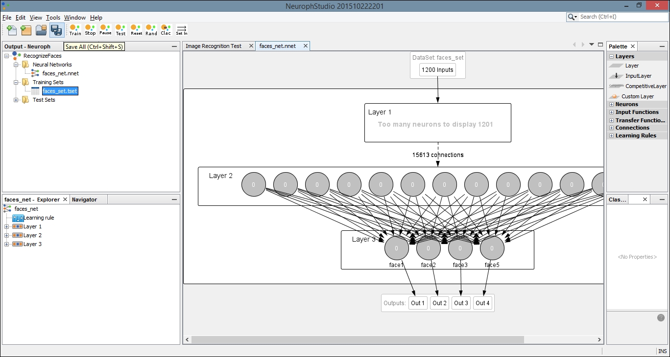
Once we have created our network, we need to train it. Begin by double-clicking on your neural network in the left pane. This is the file with the .nnet extension. When you do this, you will open a visual representation of the network in the main window. Then drag the dataset, with the file extension .tsest, from the left pane to the top node of the neural network. You will notice the description on the node change to the name of your dataset. Next, click the Train button, located in the top-left part of the window:
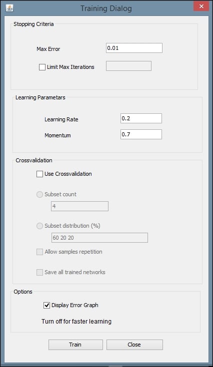
This will open a dialog box with settings for the training. You can leave the default values for Max Error, Learning Rate, and Momentum. Make sure the Display Error Graph box is checked. This allows you to see the improvement in the error rate as the training process continues:
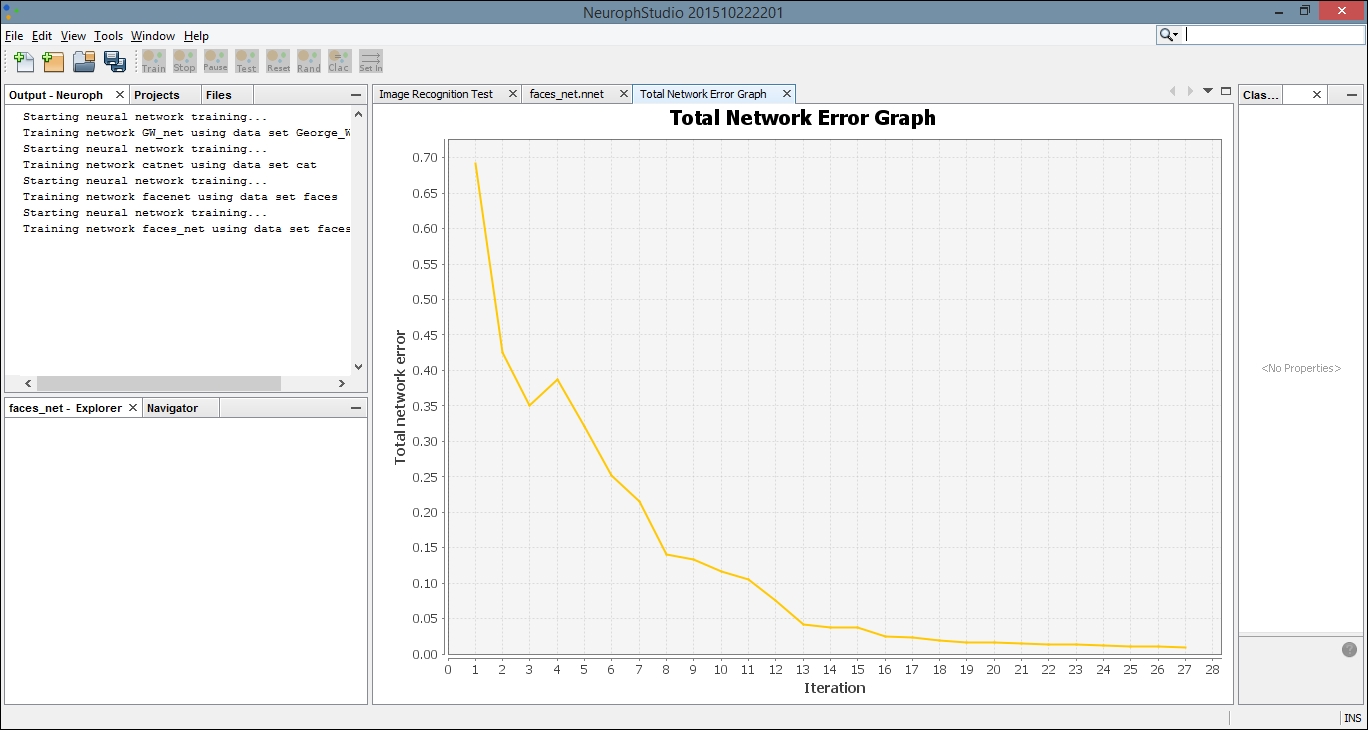
After you click the Train button, you should see an error graph similar to the following one:
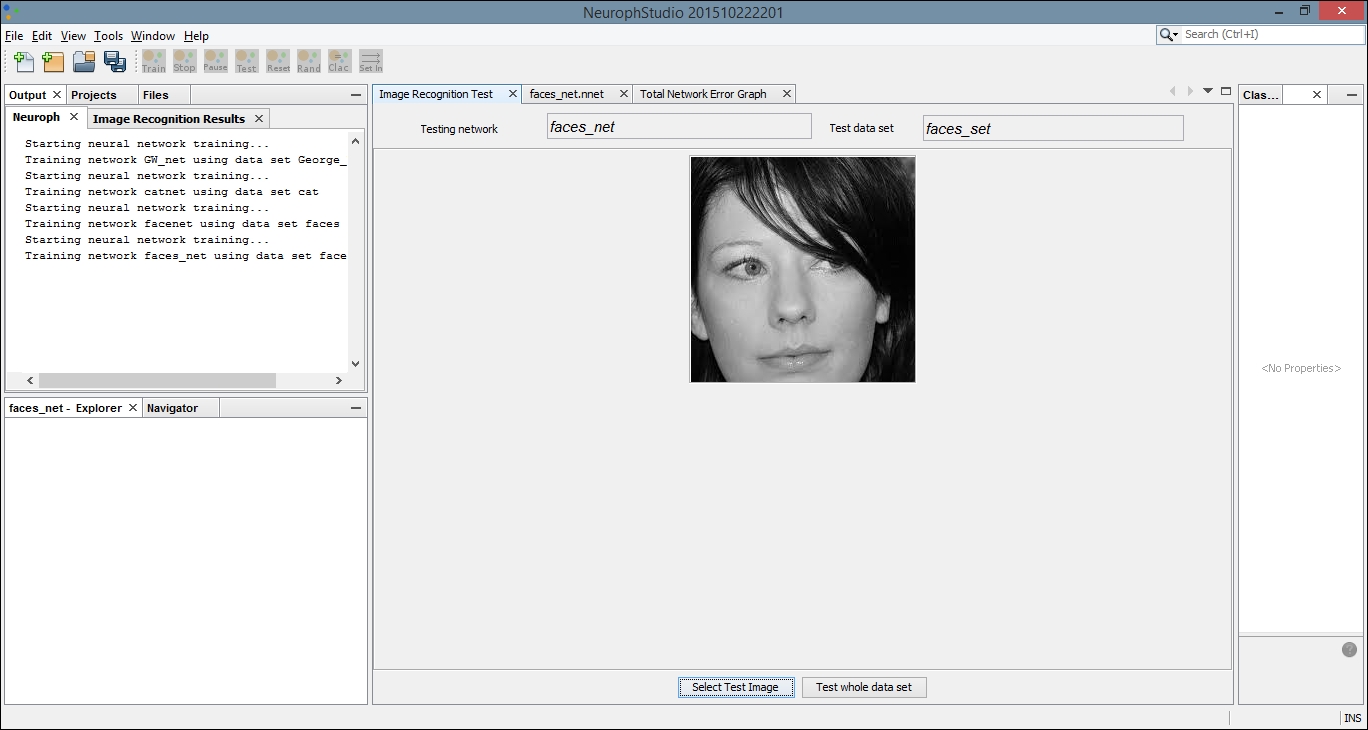
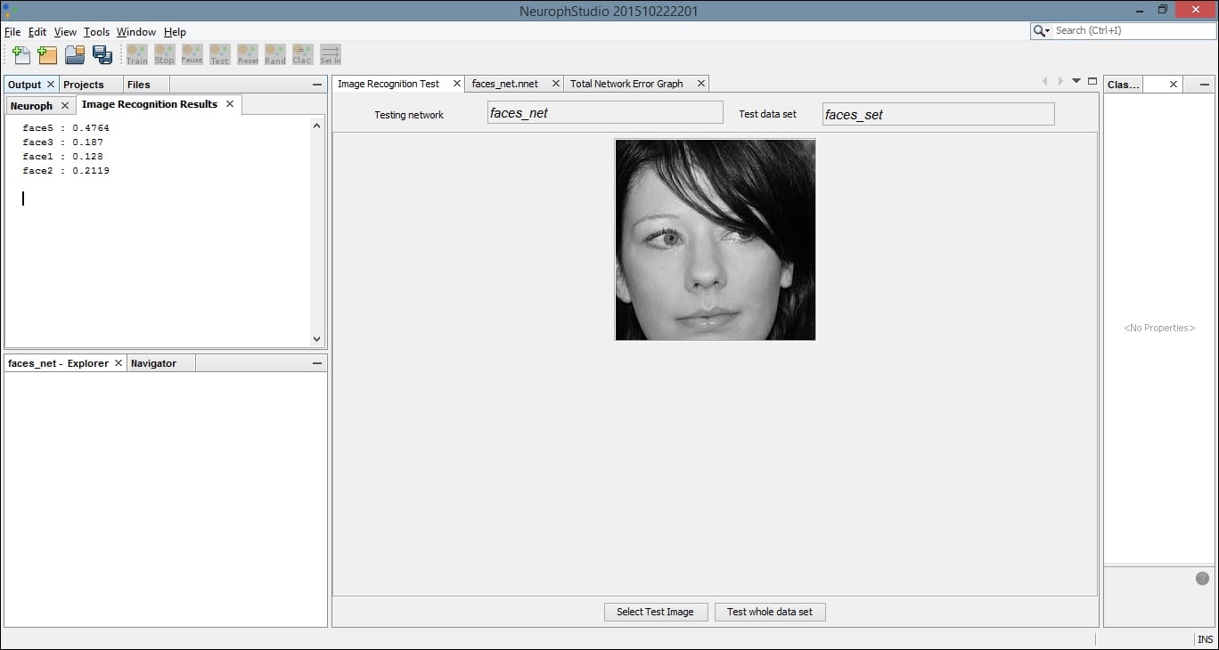
Select the tab titled Image Recognition Test. Then click on the Select Test Image button. We have loaded a simple image of a face that was not included in our original dataset:
Locate the Output tab. It will be in the bottom or left pane and will display the results of comparing our test image with each image in the training set. The greater the number, the more closely our test image matches the image from our training set. The last image results in a greater output number than the first few comparisons. If we compare these images, they are more similar than the others in the dataset, and thus the network was able to create a more positive recognition of our test image:
We can now save our network for later use. Select Save from the File menu and then you can use the .nnet file in external applications. The following code example shows a simple technique for running test data through your pre-built neural network. The NeuralNetwork class is part of the Neuroph core package, and the load method allows you to load the trained network into your project. Notice we used our neural network name, faces_net. We then retrieve the plugin for our image recognition file. Next, we call the recognizeImage method with a new image, which must handle an IOException. Our results are stored in a HashMap and printed to the console:
NeuralNetwork iRNet = NeuralNetwork.load("faces_net.nnet");
ImageRecognitionPlugin iRFile
= (ImageRecognitionPlugin)iRNet.getPlugin(
ImageRecognitionPlugin.class);
try {
HashMap<String, Double> newFaceMap
= imageRecognition.recognizeImage(
new File("testFace.jpg"));
out.println(newFaceMap.toString());
} catch(IOException e) {
// Handle exceptions
}
This process allows us to use a GUI editor application to create our network in a more visual environment, but then embed the trained network into our own applications.
Creating a Neuroph Studio project for classifying visual images
To begin, first create a new Neuroph Studio project:
We will name our project RecognizeFaces because we are going train the neural network to recognize images of human faces:
Next, we create a new file in our project. There are many types of project to choose from, but we will choose an Image Recognition type:
Click Next and then click Add directory. We have created a directory on our local machine and added several different black and white images of faces to use for training. These can be found by searching Google images or another search engine. The more quality images you have to train with, theoretically, the better your network will be:
After you click Next, you will be directed to select an image to not recognize. You may need to try different images based upon the images you want to recognize. The image you select here will prevent false recognitions. We have chosen a simple blue square from another directory on our local machine, but if you are using other types of image for training, other color blocks may work better:
Next, we need to provide network training parameters. We also need to label our training dataset and set our resolution. A height and width of 20 is a good place to start, but you may want to change these values to improve your results. Some trial and error may be involved. The purpose of providing this information is to allow for image scaling. When we scale images to a smaller size, our network can process them and learn faster:
Finally, we can create our network. We assign a label to our network and define our Transfer function. The default function, Sigmoid, will work for most networks, but if your results are not optimal you may want to try Tanh. The default number of Hidden Layers Neuron Counts is 12, and that is a good place to start. Be aware that increasing the number of neurons increases the time it takes to train the network and decreases your ability to generalize the network to other images. As with some of our previous values, some trial and error may be necessary to find the optimal settings for a given network. Select Finish when you are done:
Once we have created our network, we need to train it. Begin by double-clicking on your neural network in the left pane. This is the file with the .nnet extension. When you do this, you will open a visual representation of the network in the main window. Then drag the dataset, with the file extension .tsest, from the left pane to the top node of the neural network. You will notice the description on the node change to the name of your dataset. Next, click the Train button, located in the top-left part of the window:
This will open a dialog box with settings for the training. You can leave the default values for Max Error, Learning Rate, and Momentum. Make sure the Display Error Graph box is checked. This allows you to see the improvement in the error rate as the training process continues:
After you click the Train button, you should see an error graph similar to the following one:
Select the tab titled Image Recognition Test. Then click on the Select Test Image button. We have loaded a simple image of a face that was not included in our original dataset:
Locate the Output tab. It will be in the bottom or left pane and will display the results of comparing our test image with each image in the training set. The greater the number, the more closely our test image matches the image from our training set. The last image results in a greater output number than the first few comparisons. If we compare these images, they are more similar than the others in the dataset, and thus the network was able to create a more positive recognition of our test image:
We can now save our network for later use. Select Save from the File menu and then you can use the .nnet file in external applications. The following code example shows a simple technique for running test data through your pre-built neural network. The NeuralNetwork class is part of the Neuroph core package, and the load method allows you to load the trained network into your project. Notice we used our neural network name, faces_net. We then retrieve the plugin for our image recognition file. Next, we call the recognizeImage method with a new image, which must handle an IOException. Our results are stored in a HashMap and printed to the console:
NeuralNetwork iRNet = NeuralNetwork.load("faces_net.nnet");
ImageRecognitionPlugin iRFile
= (ImageRecognitionPlugin)iRNet.getPlugin(
ImageRecognitionPlugin.class);
try {
HashMap<String, Double> newFaceMap
= imageRecognition.recognizeImage(
new File("testFace.jpg"));
out.println(newFaceMap.toString());
} catch(IOException e) {
// Handle exceptions
}
This process allows us to use a GUI editor application to create our network in a more visual environment, but then embed the trained network into our own applications.
Training the model
Once we have created our network, we need to train it. Begin by double-clicking on your neural network in the left pane. This is the file with the .nnet extension. When you do this, you will open a visual representation of the network in the main window. Then drag the dataset, with the file extension .tsest, from the left pane to the top node of the neural network. You will notice the description on the node change to the name of your dataset. Next, click the Train button, located in the top-left part of the window:
This will open a dialog box with settings for the training. You can leave the default values for Max Error, Learning Rate, and Momentum. Make sure the Display Error Graph box is checked. This allows you to see the improvement in the error rate as the training process continues:
After you click the Train button, you should see an error graph similar to the following one:
Select the tab titled Image Recognition Test. Then click on the Select Test Image button. We have loaded a simple image of a face that was not included in our original dataset:
Locate the Output tab. It will be in the bottom or left pane and will display the results of comparing our test image with each image in the training set. The greater the number, the more closely our test image matches the image from our training set. The last image results in a greater output number than the first few comparisons. If we compare these images, they are more similar than the others in the dataset, and thus the network was able to create a more positive recognition of our test image:
We can now save our network for later use. Select Save from the File menu and then you can use the .nnet file in external applications. The following code example shows a simple technique for running test data through your pre-built neural network. The NeuralNetwork class is part of the Neuroph core package, and the load method allows you to load the trained network into your project. Notice we used our neural network name, faces_net. We then retrieve the plugin for our image recognition file. Next, we call the recognizeImage method with a new image, which must handle an IOException. Our results are stored in a HashMap and printed to the console:
NeuralNetwork iRNet = NeuralNetwork.load("faces_net.nnet");
ImageRecognitionPlugin iRFile
= (ImageRecognitionPlugin)iRNet.getPlugin(
ImageRecognitionPlugin.class);
try {
HashMap<String, Double> newFaceMap
= imageRecognition.recognizeImage(
new File("testFace.jpg"));
out.println(newFaceMap.toString());
} catch(IOException e) {
// Handle exceptions
}
This process allows us to use a GUI editor application to create our network in a more visual environment, but then embed the trained network into our own applications.
In this chapter, we demonstrated many techniques for processing speech and images. This capability is becoming important, as electronic devices are increasingly embracing these communication mediums.
TTS was demonstrated using FreeTSS. This technique allows a computer to present results as speech as opposed to text. We learned how we can control the attributes of the voice used, such as its gender and age.
Recognizing speech is useful and helps bridge the human-computer interface gap. We demonstrated how CMUSphinx is used to recognize human speech. As there is often more than one way speech can be interpreted, we learned how the API can return various options. We also demonstrated how individual words are extracted, along with the relative confidence that the right word was identified.
Image processing is a critical aspect of many applications. We started our discussion of image processing by use Tess4J to extract text from an image. This process is sometimes referred to as OCR. We learned, as with many visual and audio data files, that the quality of the results is related to the quality of the image.
We also learned how to use OpenCV to identify faces within an image. Information about specific view of faces, such as frontal or profile views, are contained in XML files. These files were used to outline faces within an image. More than one face can be detected at a time.
It can be helpful to classify images and sometimes external tools are useful for this purpose. We examined Neuroph Studio and created a neural network designed to recognize and classify images. We then tested our network with images of human faces.
In the next chapter, we will learn how to speed up common data science applications using multiple processors.