

Introduction to k-means Clustering
Hopefully, by now, you can see that finding clusters is extremely valuable in a machine learning workflow. But, how can you actually find these clusters? One of the most basic yet popular approaches is to use a cluster analysis technique called k-means clustering. The k-means clustering works by searching for k clusters in your data and the workflow is actually quite intuitive. We will start with the no-math introduction to k-means, followed by an implementation in Python. Cluster membership refers to where the points go as the algorithm processes the data. Consider it like choosing players for a sports team, where all the players are in a pool but, for each successive run, the player is assigned to a team (in this case, a cluster).
No-Math k-means Walkthrough
The no-math algorithm for k-means clustering is pretty simple:
- First, we'll pick "k" centroids, where "k" would be the expected distinct number of clusters. The value of k will be chosen by us and determines the type of clustering we obtain.
- Then, we will place the "k" centroids at random places among the existing training data.
- Next, the distance from each centroid to all the points in the training data will be calculated. We will go into detail about distance functions shortly, but for now, let's just consider it as how far points are from each other.
- Now, all the training points will be grouped with their nearest centroid.
- Isolating the grouped training points along with their respective centroid, calculate the mean data point in the group and move the previous centroid to the mean location.
- This process is to be repeated until convergence or until maximum iteration limit has been achieved.
And that's it. The following image represents original raw data:
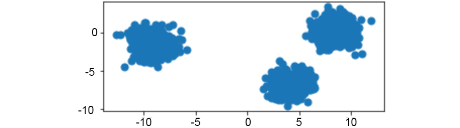
Figure 1.11: Original raw data charted on x and y coordinates
Provided with the original data in the preceding image, we can visualize the iterative process of k-means by showing the predicted clusters in each step:
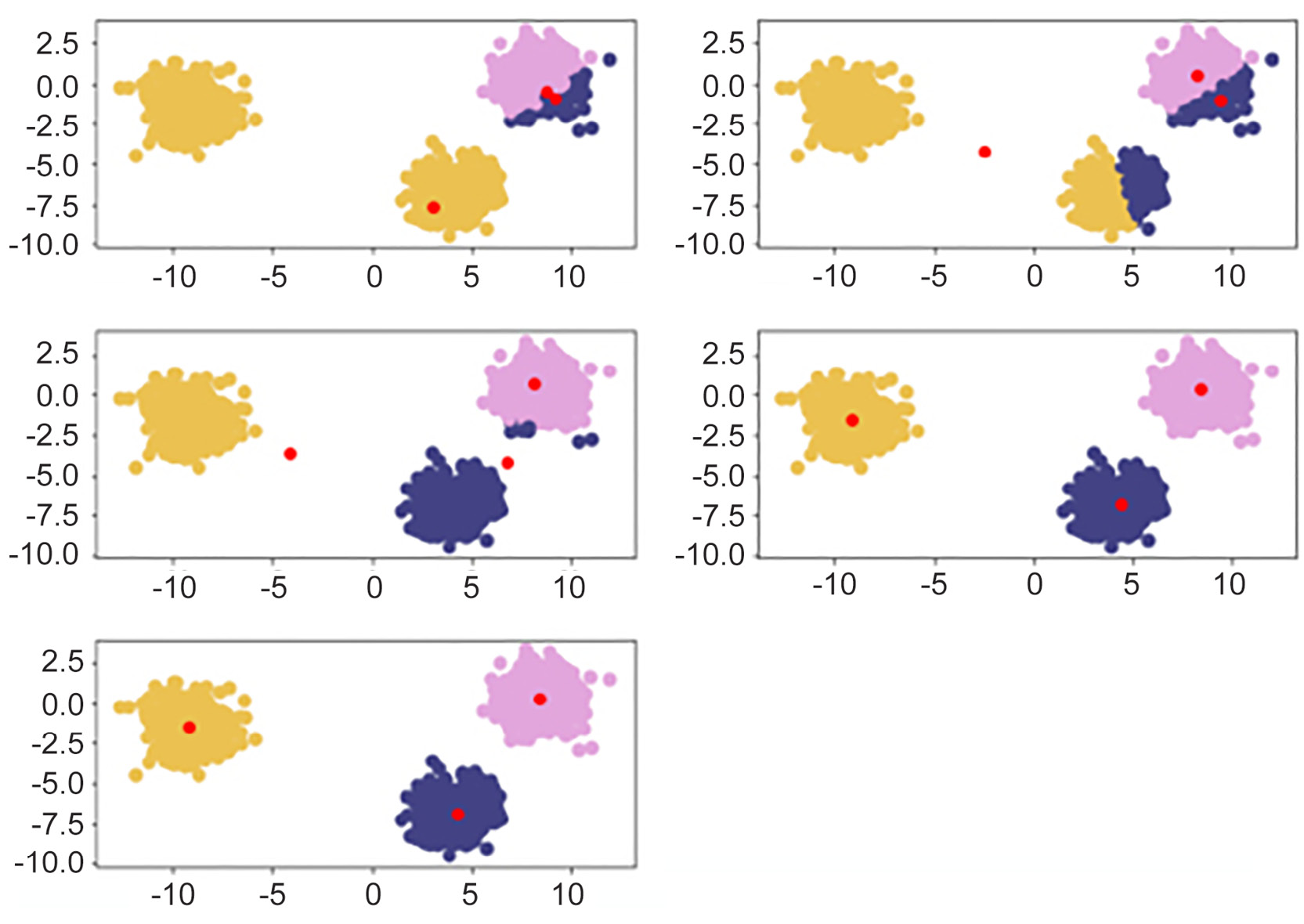
Figure 1.12: Reading from left to right, red points are randomly initialized centroids, and the closest data points are assigned to groupings of each centroid
K-means Clustering In-Depth Walkthrough
To understand k-means at a deeper level, let's walk through the example that was provided in the introduction again with some of the math that supports k-means. The most important math that underpins this algorithm is the distance function. A distance function is basically any formula that allows you to quantitatively understand how far one object is from another, with the most popular one being the Euclidean distance formula. This formula works by subtracting the respective components of each point and squaring to remove negatives, followed by adding the resulting distances and square rooting them:

Figure 1.13: Euclidean distance formula
If you notice, the preceding formula holds true for data points having only two dimensions (the number of co-ordinates). A generic way of representing the preceding equation for higher-dimensional points is as follows:

Figure 1.14: Euclidean distance formula for higher dimensional points
Let's see the terms involved in calculation of Euclidean distance between two points p and q in a higher dimensional space. Here, n is the number of dimensions of the two points. We compute the difference between the respective components of points p and q (pi and qi are known as the ith component of point p and q respectively) and square each of them. This squared value of the difference is summed up for all n components, and then square root of this sum is obtained. This value represents the Euclidean distance between point p and q. If you substitute n = 2 in the preceding equation, it will decompose to the equation represented in Figure 1.13.
Now coming back again to our discussion on k-means. Centroids are randomly set at the beginning as points in your n-dimensional space. Each of these centers is fed into the preceding formula as (a, b), and a point in your space is fed in as (x, y). Distances are calculated between each point and the coordinates of every centroid, with the centroid the shortest distance away chosen as the point's group.
As an example, let's pick three random centroids, an arbitrary point, and, using the Euclidean distance formula, calculate the distance from each point to the centroid:
- Random centroids: [ (2,5), (8,3), (4,5) ].
- Arbitrary point x: (0, 8).
- Distance from point to each centroid: [ 3.61, 9.43, 5.00 ].
Since the arbitrary point x is closest to the first centroid, it will be assigned to the first centroid.
Alternative Distance Metric – Manhattan Distance
Euclidean distance is the most common distance metric for many machine learning applications and is often known colloquially as the distance metric; however, it is not the only, or even the best, distance metric for every situation. Another popular distance metric that can be used for clustering is Manhattan distance.
Manhattan distance is called as such because it mirrors the concept of traveling through a metropolis (such as New York City) that has many square blocks. Euclidean distance relies on diagonals due to its basis in Pythagorean theorem, while Manhattan distance constrains distance to only right angles. The formula for Manhattan distance is as follows:

Figure 1.15: Manhattan distance formula
Here pi and qi are the ith component of points p and q, respectively. Building upon our examples of Euclidean distance, where we want to find the distance between two points, if our two points were (1,2) and (2,3), then the Manhattan distance would equal |1-2| + |2-3| = 1 + 1 = 2. This functionality scales to any number of dimensions. In practice, Manhattan distance may outperform Euclidean distance when it comes to high dimensional data.
Deeper Dimensions
The preceding examples can be clearly visualized when your data is only two-dimensional. This is for convenience, to help drive the point home of how k-means works and could lead you into a false understanding of how easy clustering is. In many of your own applications, your data will likely be orders of magnitude larger to the point that it cannot be perceived by visualization (anything beyond three dimensions will be unperceivable to humans). In the previous examples, you could mentally work out a few two-dimensional lines to separate the data into its own groups. At higher dimensions, you will need to be aided by a computer to find an n-dimensional hyperplane that adequately separates the dataset. In practice, this is where clustering methods such as k-means provide significant value. The following image shows the two-dimensional, three-dimensional, and n-dimensional plots:
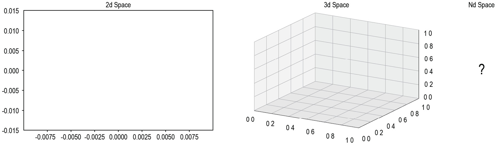
Figure 1.16: Two-dimensional, three-dimensional, and n-dimensional plots
In the next exercise, we will calculate Euclidean distance. We'll build our set of tools by using the NumPy and Math Python packages. NumPy is a scientific computing package for Python that pre-packages common mathematical functions in highly optimized formats.
As the name implies, the Math package is a basic library that makes implementing foundational math building blocks, such as exponentials and square roots, much easier. By using a package such as NumPy or Math, we help cut down the time spent creating custom math functions from scratch and instead focus on developing our solutions. You will see how each of these packages is used in practice in the following exercise.
Exercise 1.02: Calculating Euclidean Distance in Python
In this exercise, we will create an example point along with three sample centroids to help illustrate how Euclidean distance works. Understanding this distance formula is the basis for the rest of our work in clustering.
Perform the following steps to complete this exercise:
- Open a Jupyter notebook and create a naïve formula that captures the direct math of Euclidean distance, as follows:
import math
import numpy as np
def dist(a, b):
    return math.sqrt(math.pow(a[0]-b[0],2) \
                     + math.pow(a[1]-b[1],2))
Note
The code snippet shown here uses a backslash (
\) to split the logic across multiple lines. When the code is executed, Python will ignore the backslash, and treat the code on the next line as a direct continuation of the current line.This approach is considered naïve because it performs element-wise calculations on your data points (slow) compared to a more real-world implementation using vectors and matrix math to achieve significant performance increases.
- Create the data points in Python as follows:
centroids = [ (2, 5), (8, 3), (4,5) ]
x = (0, 8)
- Use the formula you created to calculate the Euclidean distance in Step 1:
# Calculating Euclidean Distance between x and centroid
centroid_distances =[]
for centroid in centroids:
    print("Euclidean Distance between x {} and centroid {} is {}"\
          .format(x ,centroid, dist(x,centroid)))
    centroid_distances.append(dist(x,centroid))
Note
The
#symbol in the code snippet above denotes a code comment. Comments are added into code to help explain specific bits of logic.The output is as follows:
Euclidean Distance between x (0, 8) and centroid (2, 5)
is 3.605551275463989
Euclidean Distance between x (0, 8) and centroid (8, 3)
is 9.433981132056603
Euclidean Distance between x (0, 8) and centroid (4, 5) is 5.0
The shortest distance between our point,
x, and the centroids is3.61, which is equivalent to the distance between(0, 8)and(2, 5). Since this is the minimum distance, our example point,x, will be assigned as a member of the first centroid's group.
In this example, our formula was used on a single point, x (0, 8). Beyond this single point, the same process will be repeated for every remaining point in your dataset until each point is assigned to a cluster. After each point is assigned, the mean point is calculated among all of the points within each cluster. The calculation of the mean among these points is the same as calculating the mean between single integers.
While there was only one point in this example, by completing this process, you have effectively assigned a point to its first cluster using Euclidean distance. We'll build upon this approach with more than one point in the following exercise.
Note
To access the source code for this specific section, please refer to https://packt.live/2VUvCuz.
You can also run this example online at https://packt.live/3ebDwpZ.
Exercise 1.03: Forming Clusters with the Notion of Distance
It is very intuitive for our human minds to see groups of dots on a plot and determine which dots belong to discrete clusters. However, how do we ask a computer to repeat this same task? In this exercise, you'll help teach a computer an approach to forming clusters of its own with the notion of distance. We will build upon how we use these distance metrics in the next exercise:
- Create a list of points, [ (0,8), (3,8), (3,4) ], that are assigned to cluster one:
cluster_1_points =[ (0,8), (3,8), (3,4) ]
- To find the new centroid among your list of points, calculate the mean point between all of the points. Calculation of the mean scales to infinite points, as you simply add the integers at each position and divide by the total number of points. For example, if your two points are (0,1,2) and (3,4,5), the mean calculation would be [ (0+3)/2, (1+4)/2, (2+5)/2 ]:
mean =[ (0+3+3)/3, (8+8+4)/3 ]
print(mean)
The output is as follows:
[2.0, 6.666666666666667]
After a new centroid is calculated, repeat the cluster membership calculation we looked at in Exercise 1.02, Calculating Euclidean Distance in Python, and then repeat the previous two steps to find the new cluster centroid. Eventually, the new cluster centroid will be the same as the centroid before the cluster membership calculation and the exercise will be complete. How many times this repeats depends on the data you are clustering.
Once you have moved the centroid location to the new mean point of (2, 6.67), you can compare it to the initial list of centroids you entered the problem with. If the new mean point is different than the centroid that is currently in your list, you will have to go through another iteration of the preceding two exercises. Once the new mean point you calculate is the same as the centroid you started the problem with, you have completed a run of k-means and reached a point called convergence. However, in practice, sometimes the number of iterations required to reach convergence is very large and such large computations may not be practically feasible. In such cases, we need to set a maximum limit to the number of iterations. Once this iteration limit is reached, we stop further processing.
Note
To access the source code for this specific section, please refer to https://packt.live/3iJ3JiT.
You can also run this example online at https://packt.live/38CCpOG.
In the next exercise, we will implement k-means from scratch. To do this, we will start employing common packages from the Python ecosystem that will serve as building blocks for the rest of your career. One of the most popular machine learning libraries is called scikit-learn (https://scikit-learn.org/stable/user_guide.html), which has many built-in algorithms and functions to support your understanding of how the algorithms work. We will also be using functions from SciPy (https://docs.scipy.org/doc/scipy/reference/), which is a package much like NumPy and abstracts away basic scientific math functions that allow for more efficient deployment. Finally, the next exercise will introduce matplotlib (https://matplotlib.org/3.1.1/contents.html), which is a plotting library that creates graphical representations of the data you are working with.
Exercise 1.04: K-means from Scratch – Part 1: Data Generation
The next two exercises focus on the creation of exercise data and the implementation of k-means from scratch on your training data. This exercise relies on scikit-learn, an open source Python package that enables the fast prototyping of popular machine learning models. Within scikit-learn, we will be using the datasets functionality to create a synthetic blob dataset. In addition to harnessing the power of scikit-learn, we will also rely on Matplotlib, a popular plotting library for Python that makes it easy for us to visualize our data. To do this, perform the following steps:
- Import the necessary libraries:
from sklearn.datasets import make_blobs
from sklearn.cluster import KMeans
import matplotlib.pyplot as plt
import numpy as np
import math
np.random.seed(0)
%matplotlib inline
Note
You can find more details on the
KMeanslibrary at https://scikit-learn.org/stable/modules/clustering.html#k-means. - Generate a random cluster dataset to experiment on X = coordinate points, y = cluster labels, and define random centroids. We will achieve this with the
make_blobsfunction that we imported fromsklearn.datasets, which, as the name implies, generates blobs of data points.X, y = make_blobs(n_samples=1500, centers=3, \ n_features=2, random_state=800) centroids = [[-6,2],[3,-4],[-5,10]]
Here the
n_samplesparameter determines the total number of data points generated by the blobs. Thecentersparameter determines the number of centroids for the blob. Then_featureattribute defines the number of dimensions generated by the dataset. Here, the data will be two dimensional.In order to generate the same data points in all the iterations (which in turn are generated randomly) for reproducibility of results, we set the
random_stateparameter to800. Different values of therandom_stateparameter would yield different results. If we do not set therandom_stateparameter, each time on execution we will obtain different results. - Print the data:
X
The output is as follows:
array([[-3.83458347,  6.09210705],
       [-4.62571831,  5.54296865],
       [-2.87807159, -7.48754592],
       ...,
       [-3.709726  , -7.77993633],
       [-8.44553266, -1.83519866],
       [-4.68308431,  6.91780744]])
- Plot the coordinate points using the scatterplot functionality we imported from
matplotlib.pyplot. This function takes input lists of points and presents them graphically for ease of understanding. Please review thematplotlibdocumentation if you want to explore the parameters provided at a deeper level:plt.scatter(X[:, 0], X[:, 1], s=50, cmap='tab20b') plt.show()
The plot appears as follows:
Figure 1.17: Plot of the coordinates
- Print the array of
y, which is the labels provided by scikit-learn and serves as the ground truth for comparison.Note
These labels will not be known to us in practice. This is just for us to cross verify our clustering in later stages.
Use the following code to print the array:
y
The output is as follows:
array([2, 2, 1, ..., 1, 0, 2])
- Plot the coordinate points with the correct cluster labels:
plt.scatter(X[:, 0], X[:, 1], c=y,s=50, cmap='tab20b')
plt.show()
The plot appears as follows:
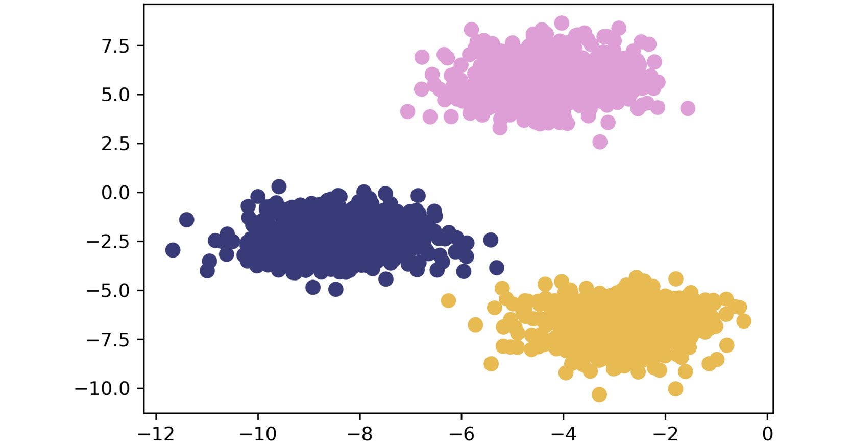
Figure 1.18: Plot of the coordinates with correct cluster labels
By completing the preceding steps, you have generated the data and visually explored how it is put together. By visualizing the ground truth, you have established a baseline that provides a relative metric for algorithm accuracy.
Note
To access the source code for this specific section, please refer to https://packt.live/2JM8Q1S.
You can also run this example online at https://packt.live/3ecjKdT.
With data in hand, in the next exercise, we'll continue by building your unsupervised learning toolset with an optimized version of the Euclidean distance function from the SciPy package, cdist. You will compare a non-vectorized, clearly understandable version of the approach with cdist, which has been specially tweaked for maximum performance.
Exercise 1.05: K-means from Scratch – Part 2: Implementing k-means
Let's recreate these results on our own. We will go over an example implementing this with some optimizations.
Note
This exercise is a continuation of the previous exercise and should be performed in the same Jupyter notebook.
For this exercise, we will rely on SciPy, a Python package that allows easy access to highly optimized versions of scientific calculations. In particular, we will be implementing Euclidean distance with cdist, the functionally of which replicates the barebones implementation of our distance metric in a much more efficient manner. Follow these steps to complete this exercise:
- The basis of this exercise will be comparing a basic implementation of Euclidean distance with an optimized version provided in SciPy. First, import the optimized Euclidean distance reference:
from scipy.spatial.distance import cdist
- Identify a subset of
Xyou want to explore. For this example, we are only selecting five points to make the lesson clearer; however, this approach scales to any number of points. We chose points 105-109, inclusive:X[105:110]
The output is as follows:
array([[-3.09897933,  4.79407445],
       [-3.37295914, -7.36901393],
       [-3.372895  ,  5.10433846],
       [-5.90267987, -3.28352194],
       [-3.52067739,  7.7841276 ]])
- Calculate the distances and choose the index of the shortest distance as a cluster:
"""
Finds distances from each of 5 sampled points to all of the centroids
"""
for x in X[105:110]:
    calcs = cdist(x.reshape([1,-1]),centroids).squeeze()
    print(calcs, "Cluster Membership: ", np.argmin(calcs))
Note
The triple-quotes (
""") shown in the code snippet above are used to denote the start and end points of a multi-line code comment. Comments are added into code to help explain specific bits of logic.The preceding code will result in the following output:
[4.027750355981394, 10.70202290628413, 5.542160268055164]
 Cluster Membership:  0
[9.73035280174993, 7.208665829113462, 17.44505393393603]
 Cluster Membership:  1
[4.066767506545852, 11.113179986633003, 5.1589701124301515]
 Cluster Membership:  0
[5.284418164665783, 8.931464028407861, 13.314157359115697]
 Cluster Membership:  0
[6.293105164930943, 13.467921029846712, 2.664298385076878]
 Cluster Membership:  2
- Define the
k_meansfunction as follows and initialize the k-centroids randomly. Repeat this process until the difference between the new/oldcentroidsequals0, using thewhileloop:Exercise1.04-Exercise1.05.ipynb
def k_means(X, K):
    # Keep track of history so you can see K-Means in action
    centroids_history = []
    labels_history = []
    rand_index = np.random.choice(X.shape[0], K)
    centroids = X[rand_index]
    centroids_history.append(centroids)
The complete code for this step can be found at https://packt.live/2JM8Q1S.
Note
Do not break this code, as it might lead to an error.
- Zip together the historical steps of centers and their labels:
history = zip(centers_hist, labels_hist)
for x, y in history:
    plt.figure(figsize=(4,3))
    plt.scatter(X[:, 0], X[:, 1], c=y, s=50, cmap='tab20b');
    plt.scatter(x[:, 0], x[:, 1], c='red')
    plt.show()
The following plots may differ from what you can see if we haven't set the random seed. The first plot looks as follows:
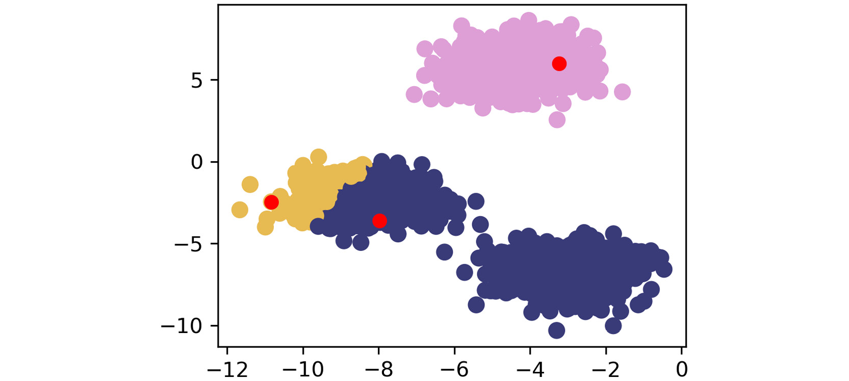
Figure 1.19: First scatterplot
The second plot appears as follows:
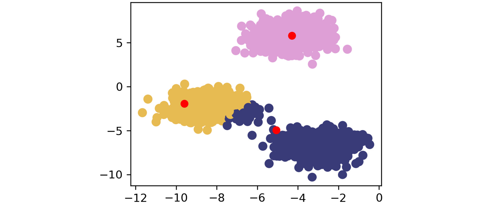
Figure 1.20: Second scatterplot
The third plot appears as follows:
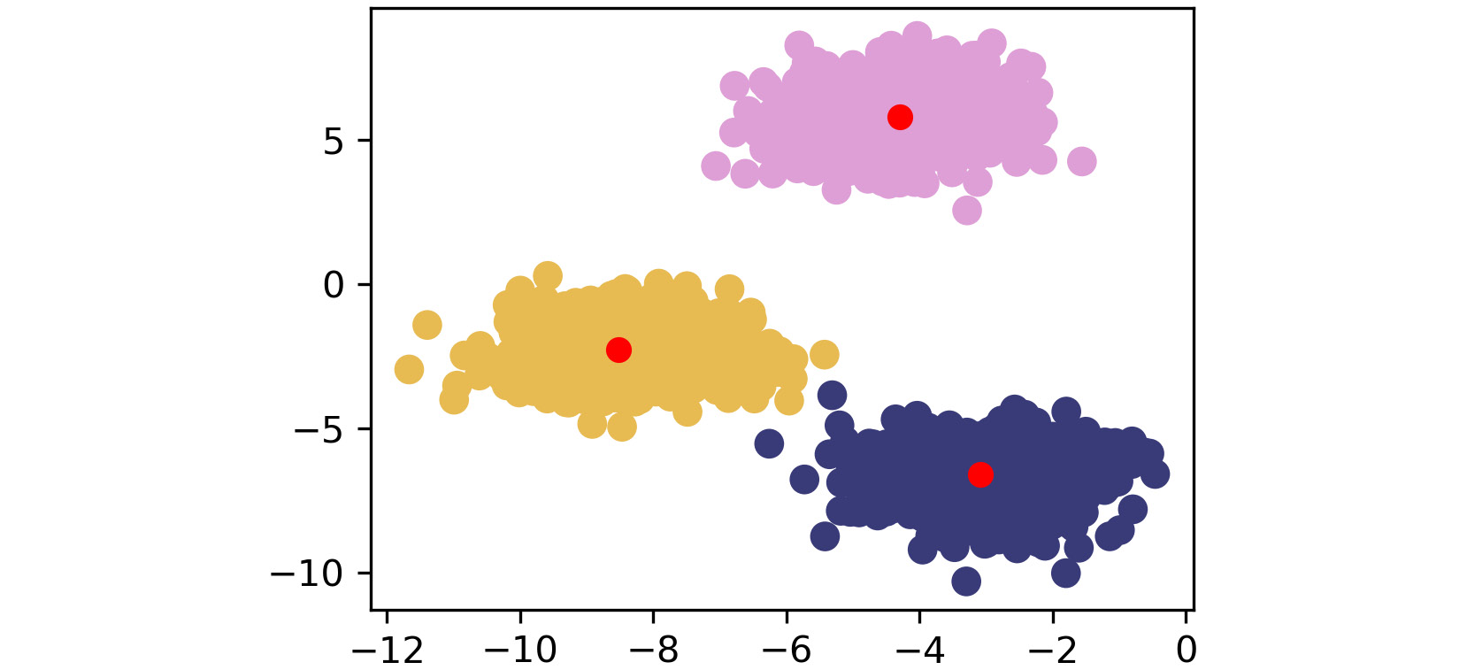
Figure 1.21: Third scatterplot
The fourth plot appears as follows:

Figure 1.22: Fourth scatterplot
The fifth plot looks as follows:
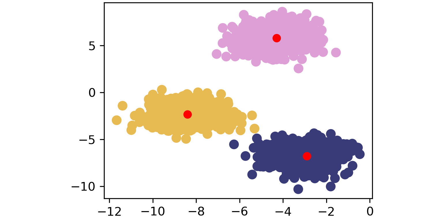
Figure 1.23: Fifth scatterplot
As shown by the preceding images, k-means takes an iterative approach to refine optimal clusters based on distance. The algorithm starts with random initialization of centroids and, depending on the complexity of the data, quickly finds the separations that make the most sense.
Note
To access the source code for this specific section, please refer to https://packt.live/2JM8Q1S.
You can also run this example online at https://packt.live/3ecjKdT.
Clustering Performance – Silhouette Score
Understanding the performance of unsupervised learning methods is inherently much more difficult than supervised learning methods because there is no ground truth available. For supervised learning, there are many robust performance metrics—the most straightforward of these being accuracy in the form of comparing model-predicted labels to actual labels and seeing how many the model got correct. Unfortunately, for clustering, we do not have labels to rely on and need to build an understanding of how "different" our clusters are. We achieve this with the silhouette score metric. We can also use silhouette scores to find the optimal "K" numbers of clusters for our unsupervised learning methods.
The silhouette metric works by analyzing how well a point fits within its cluster. The metric ranges from -1 to 1. If the average silhouette score across your clustering is one, then you will have achieved perfect clusters and there will be minimal confusion about which point belongs where. For the plots in the previous exercise, the silhouette score will be much closer to one since the blobs are tightly condensed and there is a fair amount of distance between each blob. This is very rare, though; the silhouette score should be treated as an attempt at doing the best you can, since hitting one is highly unlikely. If the silhouette score is positive, it means that a point is closer to the assigned cluster than it is to the neighboring clusters. If the silhouette score is 0, then a point lies on the boundary between the assigned cluster and the next closest cluster. If the silhouette score is negative, then it indicates that a given point is assigned to an incorrect cluster, and the given point in fact likely belongs to a neighboring cluster.
Mathematically, the silhouette score calculation is quite straightforward and is obtained using the Simplified Silhouette Index (SSI):
SSIi = bi - ai/ max(ai, bi)
Here ai is the distance from point i to its own cluster centroid, and bi is the distance from point i to the nearest cluster centroid.
The intuition captured here is that ai represents how cohesive the cluster of point i' is as a clear cluster, and bi represents how far apart the clusters lie. We will use the optimized implementation of silhouette_score in scikit-learn in Activity 1.01, Implementing k-means Clustering. Using it is simple and only requires that you pass in the feature array and the predicted cluster labels from your k-means clustering method.
In the next exercise, we will use the pandas library (https://pandas.pydata.org/pandas-docs/stable/) to read a CSV file. Pandas is a Python library that makes data wrangling easier through the use of DataFrames. If you look back at the arrays you built with NumPy, you probably noticed that the resulting data structures are quite unwieldly. To extract subsets from the data, you had to index using brackets and specific numbers of rows. Instead of this approach, pandas allows an easier-to-understand approach to moving data around and getting it into the format necessary for unsupervised learning and other machine learning techniques.
Note
To read data in Python, you will use variable_name = pd.read_csv('file_name.csv', header=None)
Here, the parameter header = None explicitly mentions that there is no presence of column names. If your file contains column names, then retain those default values. Also, if you specify header = None for a file which contains column names, Pandas will treat the row containing names of column as the row containing data only.
Exercise 1.06: Calculating the Silhouette Score
In this exercise, we will calculate the silhouette score of a dataset with a fixed number of clusters. For this, we will use the seeds dataset, which is available at https://packt.live/2UQA79z. The following note outlines more information regarding this dataset, in addition to further exploration in the next activity. For the purpose of this exercise, please disregard the specific details of what this dataset is comprised of as it is of greater importance to learn about the silhouette score. As we go into the next activity, you will gain more context as needed to create a smart machine learning system. Follow these steps to complete this exercise:
Note
This dataset is sourced from https://archive.ics.uci.edu/ml/datasets/seeds. It can be accessed at https://packt.live/2UQA79z
Citation: Contributors gratefully acknowledge support of their work by the Institute of Agrophysics of the Polish Academy of Sciences in Lublin.
- Load the seeds data file using pandas, a package that makes data wrangling much easier through the use of DataFrames:
import pandas as pd import numpy as np import matplotlib.pyplot as plt from sklearn.metrics import silhouette_score from scipy.spatial.distance import cdist np.random.seed(0) seeds = pd.read_csv('Seed_Data.csv') - Separate the
Xfeatures, since we want to treat this as an unsupervised learning problem:X = seeds[['A','P','C','LK','WK','A_Coef','LKG']]
- Bring back the
k_meansfunction we made earlier for reference:Exercise 1.06.ipynb
def k_means(X, K):
    # Keep track of history so you can see K-Means in action
    centroids_history = []
    labels_history = []
    rand_index = np.random.choice(X.shape[0], K)
    centroids = X[rand_index]
    centroids_history.append(centroids)
The complete code for this step can be found at https://packt.live/2UOqW9H.
- Convert our seeds
Xfeature DataFrame into aNumPymatrix:X_mat = X.values
- Run our
k_meansfunction on the seeds matrix:centroids, labels, centroids_history, labels_history = \ k_means(X_mat, 3)
- Calculate the silhouette score for the
Area ('A')andLength of Kernel ('LK')columns:silhouette_score(X[['A','LK']], labels)
The output should be similar to the following:
0.5875704550892767
In this exercise, we calculated the silhouette score for the Area ('A') and Length of Kernel ('LK') columns of the seeds dataset. We will use this technique in the next activity to determine the performance of our k-means clustering algorithm.
Note
To access the source code for this specific section, please refer to https://packt.live/2UOqW9H.
You can also run this example online at https://packt.live/3fbtJ4y.
Activity 1.01: Implementing k-means Clustering
You are implementing a k-means clustering algorithm from scratch to prove that you understand how it works. You will be using the seeds dataset provided by the UCI ML repository. The seeds dataset is a classic in the data science world and contains features of wheat kernels that are used to predict three different types of wheat species. The download location can be found later in this activity.
For this activity, you should use Matplotlib, NumPy, scikit-learn metrics, and pandas.
By loading and reshaping data easily, you can focus more on learning k-means instead of writing data loader functionality.
The following seeds data features are provided for reference:
1. area (A),
2. perimeter (P)
3. compactness (C)
4. length of kernel (LK)
5. width of kernel (WK)
6. asymmetry coefficient (A_Coef)
7. length of kernel groove (LKG)
The aim here is to truly understand how k-means works. To do so, you need to take what you have learned in the previous sections and implement k-means from scratch in Python.
Please open your favorite editing platform and try the following steps:
- Using
NumPyor themathpackage and the Euclidean distance formula, write a function that calculates the distance between two coordinates. - Write a function that calculates the distance from the centroids to each of the points in your dataset and returns the cluster membership.
- Write a k-means function that takes in a dataset and the number of clusters (K) and returns the final cluster centroids, as well as the data points that make up that cluster's membership. After implementing k-means from scratch, apply your custom algorithm to the seeds dataset, which is located here: https://packt.live/2Xh2FdS.
Note
This dataset is sourced from https://archive.ics.uci.edu/ml/datasets/seeds. It can be accessed at https://packt.live/2Xh2FdS.
UCI Machine Learning Repository [http://archive.ics.uci.edu/ml]. Irvine, CA: University of California, School of Information and Computer Science.
Citation: Contributors gratefully acknowledge support of their work by the Institute of Agrophysics of the Polish Academy of Sciences in Lublin.
- Remove the classes supplied in this dataset and see whether your k-means algorithm can group the different wheat species into their proper groups just based on plant characteristics!
- Calculate the silhouette score using the scikit-learn implementation.
In completing this exercise, you have gained hands-on experience of tuning a k-means clustering algorithm for a real-world dataset. The seeds dataset is seen as a classic "hello world"-type problem in the data science space and is helpful for testing foundational techniques. Your final clustering algorithm should do a decent job of finding the three clusters of wheat species types that exist in the data, as follows:
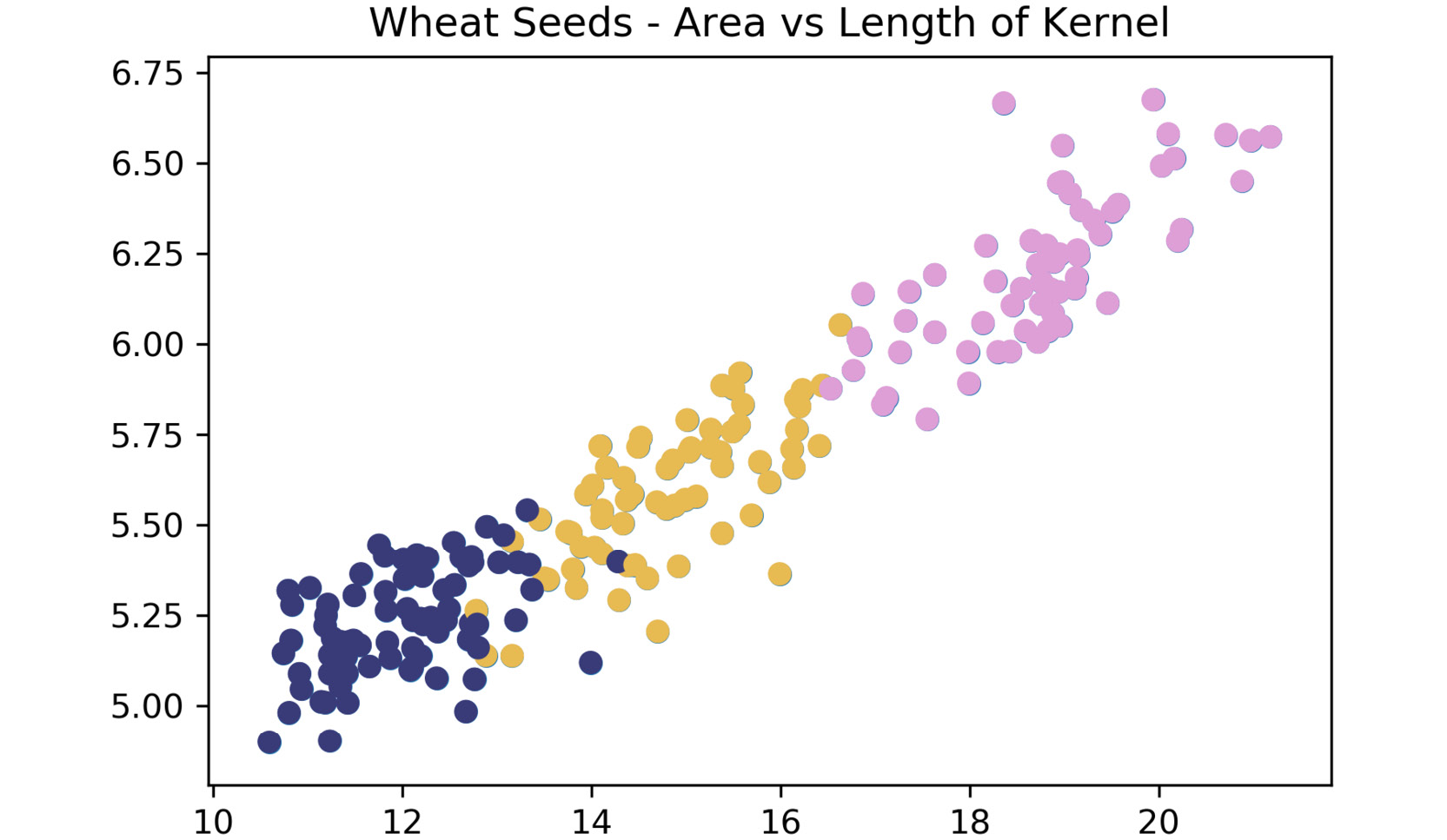
Figure 1.24: Expected plot of three clusters of wheat species
Note
The solution for this activity can be found via this link.