Sign In Start Free Trial
Account

Add to playlist

Create a Playlist

Modal Close icon
You need to login to use this feature.
  • Book Overview & Buying The Unsupervised Learning Workshop
  • Table Of Contents Toc
The Unsupervised Learning Workshop

The Unsupervised Learning Workshop

By : Aaron Jones , Richard Brooker, John Wesley Doyle , Priyanjit Ghosh, Sani Kamal, Ashish Pratik Patil , Philip Solomon, Geetank Raipuria, Christopher Kruger , Benjamin Johnston
4.3 (6)
close
close
The Unsupervised Learning Workshop

The Unsupervised Learning Workshop

4.3 (6)
By: Aaron Jones , Richard Brooker, John Wesley Doyle , Priyanjit Ghosh, Sani Kamal, Ashish Pratik Patil , Philip Solomon, Geetank Raipuria, Christopher Kruger , Benjamin Johnston

Overview of this book

Do you find it difficult to understand how popular companies like WhatsApp and Amazon find valuable insights from large amounts of unorganized data? The Unsupervised Learning Workshop will give you the confidence to deal with cluttered and unlabeled datasets, using unsupervised algorithms in an easy and interactive manner. 
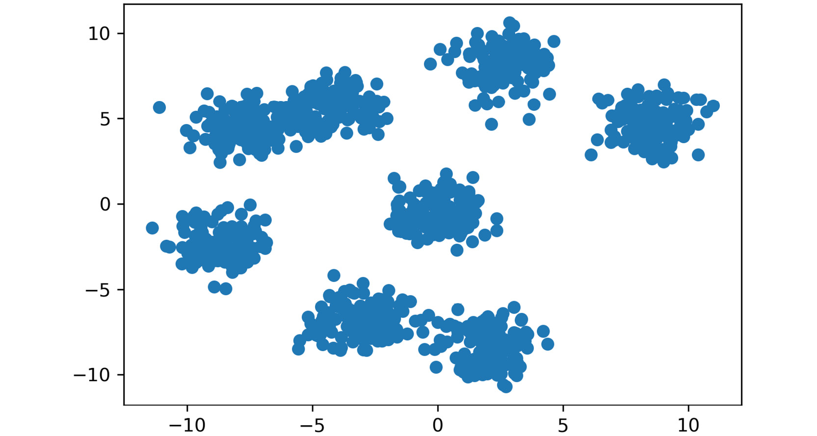
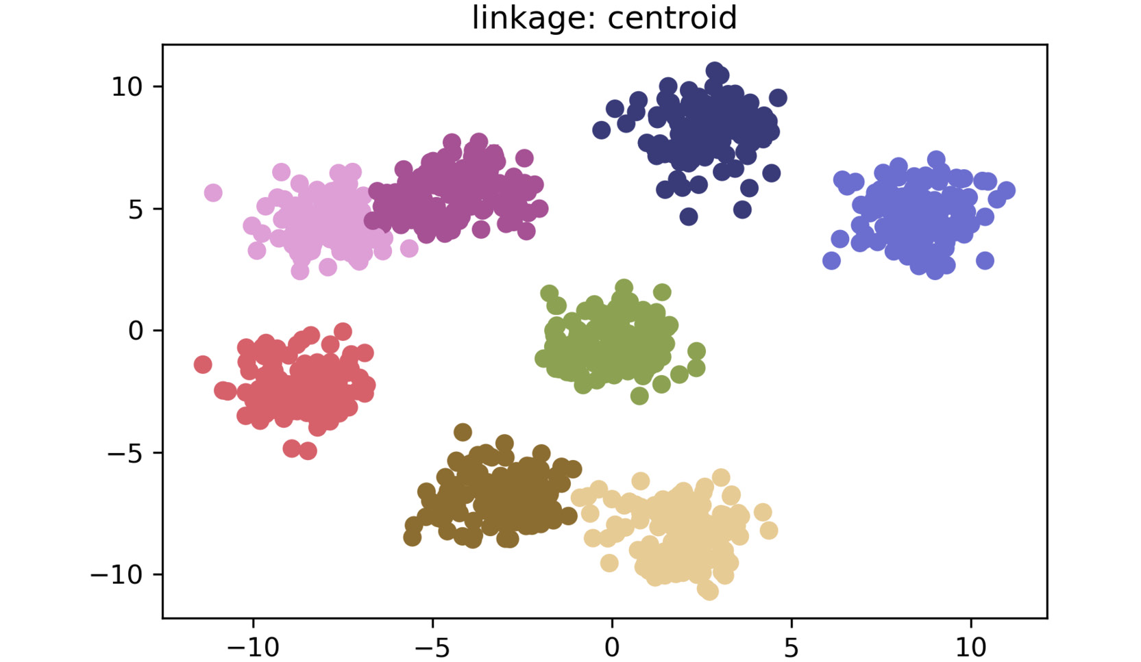
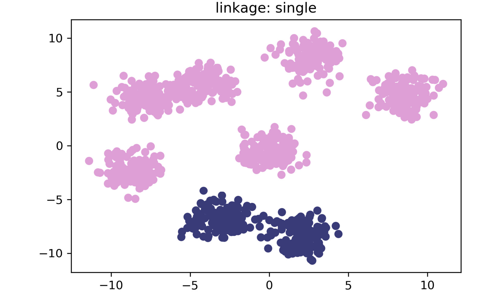
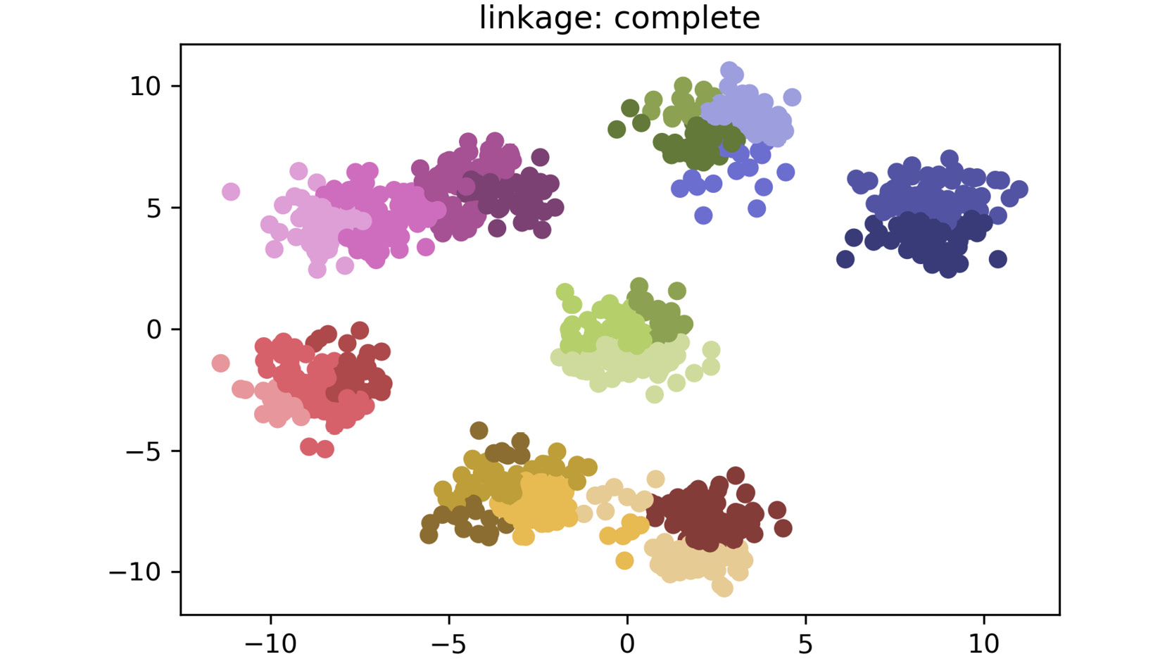
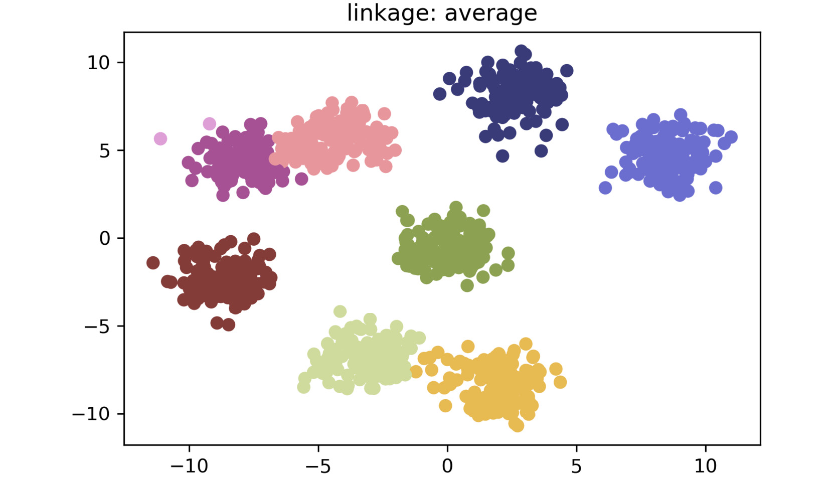
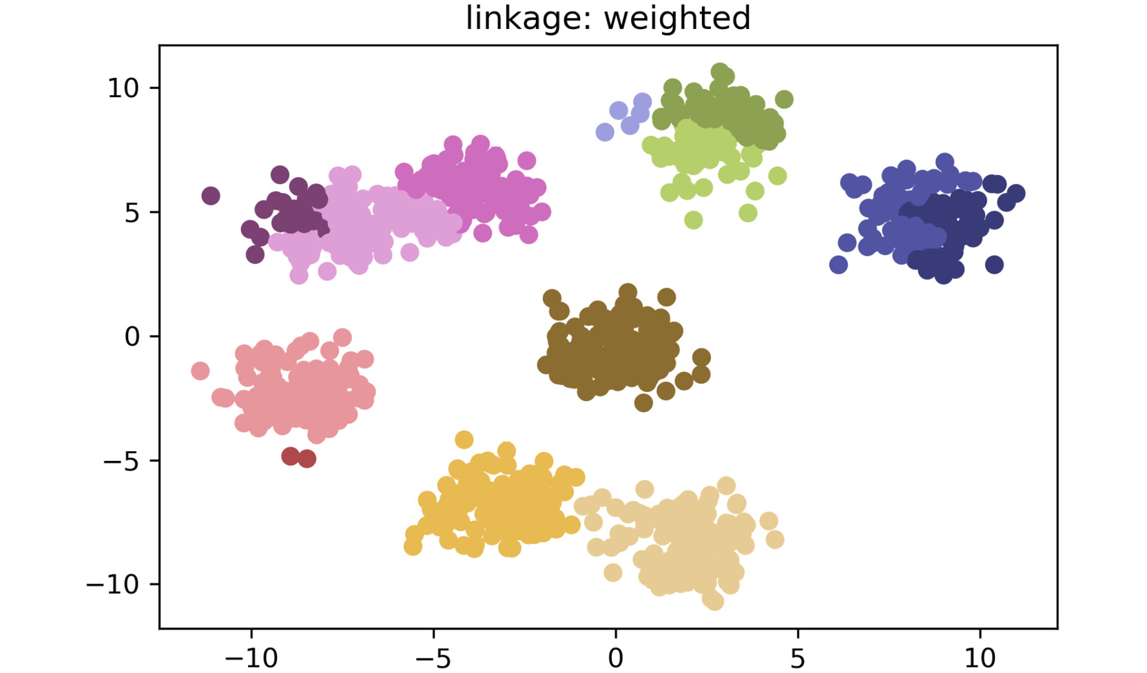
The book starts by introducing the most popular clustering algorithms of unsupervised learning. You'll find out how hierarchical clustering differs from k-means, along with understanding how to apply DBSCAN to highly complex and noisy data. Moving ahead, you'll use autoencoders for efficient data encoding. As you progress, you’ll use t-SNE models to extract high-dimensional information into a lower dimension for better visualization, in addition to working with topic modeling for implementing natural language processing (NLP). In later chapters, you’ll find key relationships between customers and businesses using Market Basket Analysis, before going on to use Hotspot Analysis for estimating the population density of an area. By the end of this book, you’ll be equipped with the skills you need to apply unsupervised algorithms on cluttered datasets to find useful patterns and insights.
Table of Contents (11 chapters)
close
close
Preface

Linkage

In Exercise 2.01, Building a Hierarchy, you implemented hierarchical clustering using what is known as Centroid Linkage. Linkage is the concept of determining how you can calculate the distances between clusters and is dependent on the type of problem you are facing. Centroid linkage was chosen for Exercise 2.02, Applying Linkage Criteria, as it essentially mirrors the new centroid search that we used in k-means. However, this is not the only option when it comes to clustering data points. Two other popular choices for determining distances between clusters are single linkage and complete linkage.

Single Linkage works by finding the minimum distance between a pair of points between two clusters as its criteria for linkage. Simply put, it essentially works by combining clusters based on the closest points between the two clusters. This is expressed mathematically as follows:

dist(a,b) = min( dist( a[i]), b[j] ) )

In the preceding code, a[i] is the ith point within first cluster where b[j] is jth point of second cluster.

Complete Linkage is the opposite of single linkage and it works by finding the maximum distance between a pair of points between two clusters as its criteria for linkage. Simply put, it works by combining clusters based on the furthest points between the two clusters. This is mathematically expressed as follows:

dist(a,b) = max( dist( a[i]), b[j] ) )

In the preceding code, a[i] and b[j] are ith and jth point of first and second cluster respectively. Determining what linkage criteria is best for your problem is as much art as it is science, and it is heavily dependent on your particular dataset. One reason to choose single linkage is if your data is similar in a nearest-neighbor sense; therefore, when there are differences, the data is extremely dissimilar. Since single linkage works by finding the closest points, it will not be affected by these distant outliers. However, as single linkage works by finding the smallest distance between a pair of points, it is quite prone to the noise distributed between the clusters. Conversely, complete linkage may be a better option if your data is distant in terms of inter-cluster state; complete linkage causes incorrect splitting when the spatial distribution of cluster is fairly imbalanced. Centroid linkage has similar benefits but falls apart if the data is very noisy and there are less clearly defined "centers" of clusters. Typically, the best approach is to try a few different linkage criteria options and see which fits your data in a way that's the most relevant to your goals.

Exercise 2.02: Applying Linkage Criteria

Recall the dummy data of the eight clusters that we generated in the previous exercise. In the real world, you may be given real data that resembles discrete Gaussian blobs in the same way. Imagine that the dummy data represents different groups of shoppers in a particular store. The store manager has asked you to analyze the shopper data in order to classify the customers into different groups so that they can tailor marketing materials to each group.

Using the data we generated in the previous exercise, or by generating new data, you are going to analyze which linkage types do the best job of grouping the customers into distinct clusters.

Once you have generated the data, view the documents supplied using SciPy to understand what linkage types are available in the linkage function. Then, evaluate the linkage types by applying them to your data. The linkage types you should test are shown in the following list:

['centroid', 'single', 'complete', 'average', 'weighted']

We haven't covered all of the previously mentioned linkage types yet – a key part of this activity is to learn how to parse the docstrings that are provided using packages to explore all of their capabilities. Follow these steps to complete this exercise:

  1. Visualize the x dataset that we created in Exercise 2.01, Building a Hierarchy:
    from scipy.cluster.hierarchy import linkage, dendrogram, fcluster
    from sklearn.datasets import make_blobs
    import matplotlib.pyplot as plt
    %matplotlib inline
  2. Generate a random cluster dataset to experiment on. X = coordinate points, y = cluster labels (not needed):
    X, y = make_blobs(n_samples=1000, centers=8, \
                      n_features=2, random_state=800)
  3. Visualize the data, as follows:
    plt.scatter(X[:,0], X[:,1])
    plt.show()

    The output is as follows:

    Figure 2.14: A scatter plot of the generated cluster dataset

    Figure 2.14: A scatter plot of the generated cluster dataset

  4. Create a list with all the possible linkage method hyperparameters:
    methods = ['centroid', 'single', 'complete', \
               'average', 'weighted']
  5. Loop through each of the methods in the list that you just created and display the effect that they have on the same dataset:
    for method in methods:
        distances = linkage(X, method=method, metric="euclidean")
        clusters = fcluster(distances, 3, criterion="distance") 
        plt.title('linkage: ' + method)
        plt.scatter(X[:,0], X[:,1], c=clusters, cmap='tab20b')
        plt.show()

    The plot for centroid linkage is as follows:

    Figure 2.15: A scatter plot for centroid linkage method

Figure 2.15: A scatter plot for centroid linkage method

The plot for single linkage is as follows:

Figure 2.16: A scatter plot for single linkage method

Figure 2.16: A scatter plot for single linkage method

The plot for complete linkage is as follows:

Figure 2.17: A scatter plot for complete linkage method

Figure 2.17: A scatter plot for complete linkage method

The plot for average linkage is as follows:

Figure 2.18: A scatter plot for average linkage method

Figure 2.18: A scatter plot for average linkage method

The plot for weighted linkage is as follows:

Figure 2.19: A scatter plot for weighted linkage method

Figure 2.19: A scatter plot for weighted linkage method

As shown in the preceding plots, by simply changing the linkage criteria, you can dramatically change the efficacy of your clustering. In this dataset, centroid and average linkage work best at finding discrete clusters that make sense. This is clear from the fact that we generated a dataset of eight clusters, and centroid and average linkage are the only ones that show the clusters that are represented using eight different colors. The other linkage types fall short – most noticeably, single linkage. Single linkage falls short because it operates on the assumption that the data is in a thin "chain" format versus the clusters. The other linkage methods are superior due to their assumption that the data is coming in as clustered groups.

Note

To access the source code for this specific section, please refer to https://packt.live/2VWwbEv.

You can also run this example online at https://packt.live/2Zb4zgN.

CONTINUE READING
83
Tech Concepts
36
Programming languages
73
Tech Tools
Icon Unlimited access to the largest independent learning library in tech of over 8,000 expert-authored tech books and videos.
Icon Innovative learning tools, including AI book assistants, code context explainers, and text-to-speech.
Icon 50+ new titles added per month and exclusive early access to books as they are being written.
The Unsupervised Learning Workshop
notes
bookmark Notes and Bookmarks search Search in title playlist Add to playlist download Download options font-size Font size

Change the font size

margin-width Margin width

Change margin width

day-mode Day/Sepia/Night Modes

Change background colour

Close icon Search
Country selected

Close icon Your notes and bookmarks

Confirmation

Modal Close icon
claim successful

Buy this book with your credits?

Modal Close icon
Are you sure you want to buy this book with one of your credits?
Close
YES, BUY

Submit Your Feedback

Modal Close icon
Modal Close icon
Modal Close icon