Text normalization

Text normalization is a pre-processing step aimed at improving the quality of the text and making it suitable for machines to process. Four main steps in text normalization are case normalization, tokenization and stop word removal, Parts-of-Speech (POS) tagging, and stemming.

Case normalization applies to languages that use uppercase and lowercase letters. All languages based on the Latin alphabet or the Cyrillic alphabet (Russian, Mongolian, and so on) use upper- and lowercase letters. Other languages that sometimes use this are Greek, Armenian, Cherokee, and Coptic. In case normalization, all letters are converted to the same case. It is quite helpful in semantic use cases. However, in other cases, this may hinder performance. In the spam example, spam messages may have more words in all-caps compared to regular messages.

Another common normalization step removes punctuation in the text. Again, this may or may not be useful given the problem at hand. In most cases, this should give good results. However, in some cases, such as spam or grammar models, it may hinder performance. It is more likely for spam messages to use more exclamation marks or other punctuation for emphasis.

Let's build a baseline model with three simple features:

• Number of characters in the message
• Number of capital letters in the message
• Number of punctuation symbols in the message

To do so, first, we will convert the data into a pandas DataFrame:

import pandas as pd
df = pd.DataFrame(spam_dataset, columns=['Spam', 'Message'])

Next, let's build some simple functions that can count the length of the message, and the numbers of capital letters and punctuation symbols. Python's regular expression package, re, will be used to implement these:

import re
def message_length(x):
  # returns total number of characters
  return len(x)
def num_capitals(x):
  _, count = re.subn(r'[A-Z]', '', x) # only works in english
  return count
def num_punctuation(x):
  _, count = re.subn(r'\W', '', x)
  return count

In the num_capitals() function, substitutions are performed for the capital letters in English. The count of these substitutions provides the count of capital letters. The same technique is used to count the number of punctuation symbols. Please note that the method used to count capital letters is specific to English.

Additional feature columns will be added to the DataFrame, and then the set will be split into test and train sets:

df['Capitals'] = df['Message'].apply(num_capitals)
df['Punctuation'] = df['Message'].apply(num_punctuation)
df['Length'] = df['Message'].apply(message_length)
df.describe()

This should generate the following output:

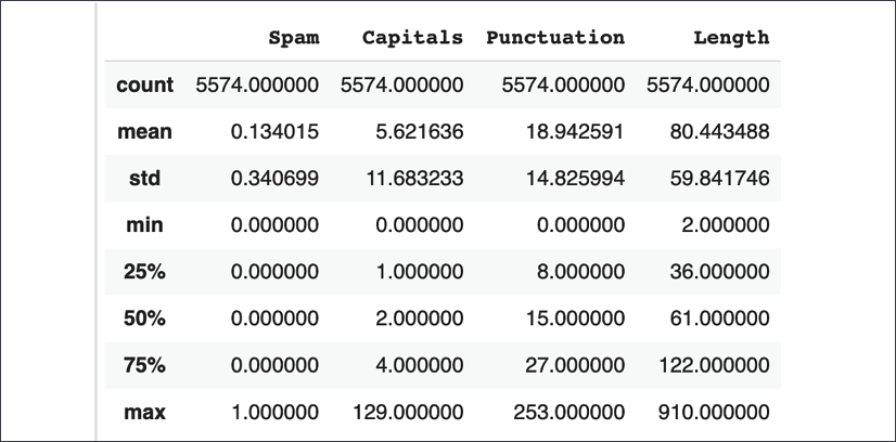
Figure 1.5: Base dataset for initial spam model

The following code can be used to split the dataset into training and test sets, with 80% of the records in the training set and the rest in the test set. Further more, labels will be removed from both the training and test sets:

train=df.sample(frac=0.8,random_state=42)
test=df.drop(train.index)
x_train = train[['Length', 'Capitals', 'Punctuation']]
y_train = train[['Spam']]
x_test = test[['Length', 'Capitals', 'Punctuation']]
y_test = test[['Spam']]

Now we are ready to build a simple classifier to use this data.

Modeling normalized data

Recall that modeling was the last part of the text processing pipeline described earlier. In this chapter, we will use a very simple model, as the objective is to show different basic NLP data processing techniques more than modeling. Here, we want to see if three simple features can aid in the classification of spam. As more features are added, passing them through the same model will help in seeing if the featurization aids or hampers the accuracy of the classification.

A function is defined that allows the construction of models with different numbers of inputs and hidden units:

# Basic 1-layer neural network model for evaluation
def make_model(input_dims=3, num_units=12):
  model = tf.keras.Sequential()
  # Adds a densely-connected layer with 12 units to the model:
  model.add(tf.keras.layers.Dense(num_units, 
                                  input_dim=input_dims,
                                  activation='relu'))
  # Add a sigmoid layer with a binary output unit:
  model.add(tf.keras.layers.Dense(1, activation='sigmoid'))
  model.compile(loss='binary_crossentropy', optimizer='adam', 
                metrics=['accuracy'])
  return model

This model uses binary cross-entropy for computing loss and the Adam optimizer for training. The key metric, given that this is a binary classification problem, is accuracy. The default parameters passed to the function are sufficient as only three features are being passed in.

We can train our simple baseline model with only three features like so:

model = make_model()
model.fit(x_train, y_train, epochs=10, batch_size=10)

Train on 4459 samples
Epoch 1/10
4459/4459 [==============================] - 1s 281us/sample - loss: 0.6062 - accuracy: 0.8141
Epoch 2/10
…
Epoch 10/10
4459/4459 [==============================] - 1s 145us/sample - loss: 0.1976 - accuracy: 0.9305

This is not bad as our three simple features help us get to 93% accuracy. A quick check shows that there are 592 spam messages in the test set, out of a total of 4,459. So, this model is doing better than a very simple model that guesses everything as not spam. That model would have an accuracy of 87%. This number may be surprising but is fairly common in classification problems where there is a severe class imbalance in the data. Evaluating it on the training set gives an accuracy of around 93.4%:

model.evaluate(x_test, y_test)

1115/1115 [==============================] - 0s 94us/sample - loss: 0.1949 - accuracy: 0.9336
[0.19485870356516988, 0.9336323]

Please note that the actual performance you see may be slightly different due to the data splits and computational vagaries. A quick verification can be performed by plotting the confusion matrix to see the performance:

y_train_pred = model.predict_classes(x_train)
# confusion matrix
tf.math.confusion_matrix(tf.constant(y_train.Spam), 
                         y_train_pred)
<tf.Tensor: shape=(2, 2), dtype=int32, numpy=
array([[3771,   96],
      [ 186,  406]], dtype=int32)>

This shows that 3,771 out of 3,867 regular messages were classified correctly, while 406 out of 592 spam messages were classified correctly. Again, you may get a slightly different result.

To test the value of the features, try re-running the model by removing one of the features, such as punctuation or a number of capital letters, to get a sense of their contribution to the model. This is left as an exercise for the reader.

Tokenization

This step takes a piece of text and converts it into a list of tokens. If the input is a sentence, then separating the words would be an example of tokenization. Depending on the model, different granularities can be chosen. At the lowest level, each character could become a token. In some cases, entire sentences of paragraphs can be considered as a token:

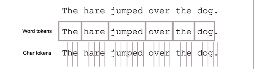
Figure 1.6: Tokenizing a sentence

The preceding diagram shows two ways a sentence can be tokenized. One way to tokenize is to chop a sentence into words. Another way is to chop into individual characters. However, this can be a complex proposition in some languages such as Japanese and Mandarin.

Segmentation in Japanese

Many languages use a word separator, a space, to separate words. This makes the task of tokenizing on words trivial. However, there are other languages that do not use any markers or separators between words. Some examples of such languages are Japanese and Chinese. In such languages, the task is referred to as segmentation.

Specifically, in Japanese, there are mainly three different types of characters that are used: Hiragana, Kanji, and Katakana. Kanji is adapted from Chinese characters, and similar to Chinese, there are thousands of characters. Hiragana is used for grammatical elements and native Japanese words. Katakana is mostly used for foreign words and names. Depending on the preceding characters, a character may be part of an existing word or the start of a new word. This makes Japanese one of the most complicated writing systems in the world. Compound words are especially hard. Consider the following compound word that reads Election Administration Committee:

This can be tokenized in two different ways, outside of the entire phrase being considered one word. Here are two examples of tokenizing (from the Sudachi library):

(Election / Administration / Committee)

(Election / Administration / Committee / Meeting)

Common libraries that are used specifically for Japanese segmentation or tokenization are MeCab, Juman, Sudachi, and Kuromoji. MeCab is used in Hugging Face, spaCy, and other libraries.

Fortunately, most languages are not as complex as Japanese and use spaces to separate words. In Python, splitting by spaces is trivial. Let's take an example:

Sentence = 'Go until Jurong point, crazy.. Available only in bugis n great world'
sentence.split()

The output of the preceding split operation results in the following:

['Go',
 'until',
 'jurong',
 'point,',
 'crazy..',
 'Available',
 'only',
 'in',
 'bugis',
 'n',
 'great',
 'world']

The two highlighted lines in the preceding output show that the naïve approach in Python will result in punctuation being included in the words, among other issues. Consequently, this step is done through a library like StanfordNLP. Using pip, let's install this package in our Colab notebook:

!pip install stanfordnlp

The StanfordNLP package uses PyTorch under the hood as well as a number of other packages. These and other dependencies will be installed. By default, the package does not install language files. These have to be downloaded. This is shown in the following code:

Import stanfordnlp as snlp
en = snlp.download('en')

The English file is approximately 235 MB. A prompt will be displayed to confirm the download and the location to store it in:

Figure 1.7: Prompt for downloading English models

This package provides capabilities for tokenization, POS tagging, and lemmatization out of the box. To start with tokenization, we instantiate a pipeline and tokenize a sample text to see how this works:

en = snlp.Pipeline(lang='en', processors='tokenize')

The lang parameter is used to indicate that an English pipeline is desired. The second parameter, processors, indicates the type of processing that is desired in the pipeline. This library can also perform the following processing steps in the pipeline:

• pos labels each token with a POS token. The next section provides more details on POS tags.
• lemma, which can convert different forms of verbs, for example, to the base form. This will be covered in detail in the Stemming and lemmatization section later in this chapter.
• depparse performs dependency parsing between words in a sentence. Consider the following example sentence, "Hari went to school." Hari is interpreted as a noun by the POS tagger, and becomes the governor of the word went. The word school is dependent on went as it describes the object of the verb.

For now, only tokenization of text is desired, so only the tokenizer is used:

tokenized = en(sentence)
len(tokenized.sentences)

2

This shows that the tokenizer correctly divided the text into two sentences. To investigate what words were removed, the following code can be used:

for snt in tokenized.sentences:
  for word in snt.tokens:
    print(word.text)
  print("<End of Sentence>")

Go
until
jurong
point
,
crazy
..
<End of Sentence>
Available
only
in
bugis
n
great
world
<End of Sentence>

Note the highlighted words in the preceding output. Punctuation marks were separated out into their own words. Text was split into multiple sentences. This is an improvement over only using spaces to split. In some applications, removal of punctuation may be required. This will be covered in the next section.

Consider the preceding example of Japanese. To see the performance of StanfordNLP on Japanese tokenization, the following piece of code can be used:

jp = snlp.download('ja')

This is the first step, which involves downloading the Japanese language model, similar to the English model that was downloaded and installed previously. Next, a Japanese pipeline will be instantiated and the words will be processed:

jp = snlp.download('ja')
jp_line = jp("")

You may recall that the Japanese text reads Election Administration Committee. Correct tokenization should produce three words, where first two should be two characters each, and the last word is three characters:

for snt in jp_line.sentences:
  for word in snt.tokens:
    print(word.text)

This matches the expected output. StanfordNLP supports 53 languages, so the same code can be used for tokenizing any language that is supported.

Coming back to the spam detection example, a new feature can be implemented that counts the number of words in the message using this tokenization functionality.

It is possible that spam messages have different numbers of words than regular messages. The first step is to define a method to compute the number of words:

en = snlp.Pipeline(lang='en')
def word_counts(x, pipeline=en):
  doc = pipeline(x)
  count = sum([len(sentence.tokens) for sentence in doc.sentences])
  return count

Next, using the train and test splits, add a column for the word count feature:

train['Words'] = train['Message'].apply(word_counts)
test['Words'] = test['Message'].apply(word_counts)
x_train = train[['Length', 'Punctuation', 'Capitals', 'Words']]
y_train = train[['Spam']]
x_test = test[['Length', 'Punctuation', 'Capitals' , 'Words']]
y_test = test[['Spam']]
model = make_model(input_dims=4)

The last line in the preceding code block creates a new model with four input features.

/pytorch/aten/src/ATen/native/LegacyDefinitions.cpp:19: UserWarning: masked_fill_ received a mask with dtype torch.uint8, this behavior is now deprecated,please use a mask with dtype torch.bool instead.

Modeling tokenized data

This model can be trained like so:

model.fit(x_train, y_train, epochs=10, batch_size=10)
Train on 4459 samples
Epoch 1/10
4459/4459 [==============================] - 1s 202us/sample - loss: 2.4261 - accuracy: 0.6961
...
Epoch 10/10
4459/4459 [==============================] - 1s 142us/sample - loss: 0.2061 - accuracy: 0.9312

There is only a marginal improvement in accuracy. One hypothesis is that the number of words is not useful. It would be useful if the average number of words in spam messages were smaller or larger than regular messages. Using pandas, this can be quickly verified:

train.loc[train.Spam == 1].describe()

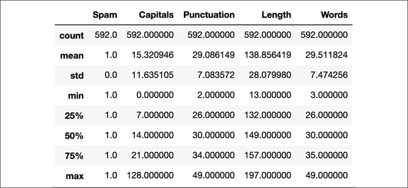
Figure 1.8: Statistics for spam message features

Let's compare the preceding results to the statistics for regular messages:

train.loc[train.Spam == 0].describe()

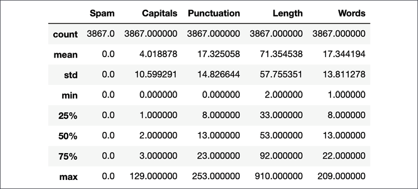
Figure 1.9: Statistics for regular message features

Some interesting patterns can quickly be seen. Spam messages usually have much less deviation from the mean. Focus on the Capitals feature column. It shows that regular messages use far fewer capitals than spam messages. At the 75^th percentile, there are 3 capitals in a regular message versus 21 for spam messages. On average, regular messages have 4 capital letters while spam messages have 15. This variation is much less pronounced in the number of words category. Regular messages have 17 words on average, while spam has 29. At the 75^th percentile, regular messages have 22 words while spam messages have 35. This quick check yields an indication as to why adding the word features wasn't that useful. However, there are a couple of things to consider still. First, the tokenization model split out punctuation marks as words. Ideally, these words should be removed from the word counts as the punctuation feature is showing that spam messages use a lot more punctuation characters. This will be covered in the Parts-of-speech tagging section. Secondly, languages have some common words that are usually excluded. This is called stop word removal and is the focus of the next section.

Stop word removal

Stop word removal involves removing common words such as articles (the, an) and conjunctions (and, but), among others. In the context of information retrieval or search, these words would not be helpful in identifying documents or web pages that would match the query. As an example, consider the query "Where is Google based?". In this query, is is a stop word. The query would produce similar results irrespective of the inclusion of is. To determine the stop words, a simple approach is to use grammar clues.

In English, articles and conjunctions are examples of classes of words that can usually be removed. A more robust way is to consider the frequency of occurrence of words in a corpus, set of documents, or text. The most frequent terms can be selected as candidates for the stop word list. It is recommended that this list be reviewed manually. There can be cases where words may be frequent in a collection of documents but are still meaningful. This can happen if all the documents in the collection are from a specific domain or on a specific topic. Consider a set of documents from the Federal Reserve. The word economy may appear quite frequently in this case; however, it is unlikely to be a candidate for removal as a stop word.

In some cases, stop words may actually contain information. This may be applicable to phrases. Consider the fragment "flights to Paris." In this case, to provides valuable information, and its removal may change the meaning of the fragment.

Recall the stages of the text processing workflow. The step after text normalization is vectorization. This step is discussed in detail later in the Vectorizing text section of this chapter, but the key step in vectorization is to build a vocabulary or dictionary of all the tokens. The size of this vocabulary can be reduced by removing stop words. While training and evaluating models, removing stop words reduces the number of computation steps that need to be performed. Hence, the removal of stop words can yield benefits in terms of computation speed and storage space. Modern advances in NLP see smaller and smaller stop words lists as more efficient encoding schemes and computation methods evolve. Let's try and see the impact of stop words on the spam problem to develop some intuition about its usefulness.

Many NLP packages provide lists of stop words. These can be removed from the text after tokenization. Tokenization was done through the StanfordNLP library previously. However, this library does not come with a list of stop words. NLTK and spaCy supply stop words for a set of languages. For this example, we will use an open source package called stopwordsiso.

This Python package takes the list of stop words from the stopwords-iso GitHub project at https://github.com/stopwords-iso/stopwords-iso. This package provides stop words in 57 languages. The first step is to install the Python package that provides access to the stop words lists.

The following command will install the package through the notebook:

!pip install stopwordsiso

Supported languages can be checked with the following commands:

import stopwordsiso as stopwords
stopwords.langs()

English language stop words can be checked as well to get an idea of some of the words:

sorted(stopwords.stopwords('en'))

["'ll",
 "'tis",
 "'twas",
 "'ve",
 '10',
 '39',
 'a',
 "a's",
 'able',
 'ableabout',
 'about',
 'above',
 'abroad',
 'abst',
 'accordance',
 'according',
 'accordingly',
 'across',
 'act',
 'actually',
 'ad',
 'added',
...

Given that tokenization was already implemented in the preceding word_counts() method, the implementation of that method can be updated to include removing stop words. However, all the stop words are in lowercase. Case normalization was discussed earlier, and capital letters were a useful feature for spam detection. In this case, tokens need to be converted to lowercase to effectively remove them:

en_sw = stopwords.stopwords('en')
def word_counts(x, pipeline=en):
  doc = pipeline(x)
  count = 0
  for sentence in doc.sentences:
    for token in sentence.tokens:
        if token.text.lower() not in en_sw:
          count += 1
  return count

A consequence of using stop words is that a message such as "When are you going to ride your bike?" counts as only 3 words. When we see if this has had any effect on the statistics for word length, the following picture emerges:

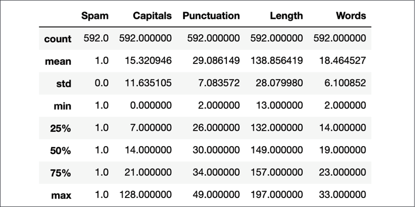
Figure 1.10: Word counts for spam messages after removing stop words

Compared to the word counts prior to stop word removal, the average number of words has been reduced from 29 to 18, almost a 30% decrease. The 25^th percentile changed from 26 to 14. The maximum has also reduced from 49 to 33.

The impact on regular messages is even more dramatic:

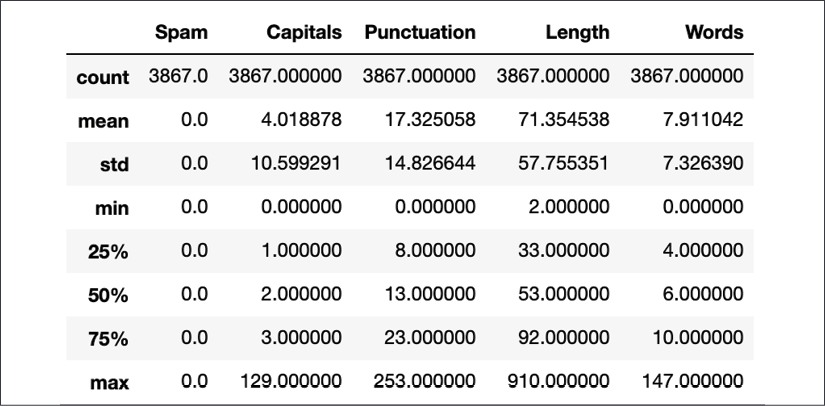
Figure 1.11: Word counts for regular messages after removing stop words

Comparing these statistics to those from before stop word removal, the average number of words has more than halved to almost 8. The maximum number of words has also reduced from 209 to 147. The standard deviation of regular messages is about the same as its mean, indicating that there is a lot of variation in the number of words in regular messages. Now, let's see if this helps us train a model and improve its accuracy.

Modeling data with stop words removed

Now that the feature without stop words is computed, it can be added to the model to see its impact:

train['Words'] = train['Message'].apply(word_counts)
test['Words'] = test['Message'].apply(word_counts)
x_train = train[['Length', 'Punctuation', 'Capitals', 'Words']]
y_train = train[['Spam']]
x_test = test[['Length', 'Punctuation', 'Capitals', 'Words']]
y_test = test[['Spam']]
model = make_model(input_dims=4)
model.fit(x_train, y_train, epochs=10, batch_size=10)

Epoch 1/10
4459/4459 [==============================] - 2s 361us/sample - loss: 0.5186 - accuracy: 0.8652
Epoch 2/10
...
Epoch 9/10
4459/4459 [==============================] - 2s 355us/sample - loss: 0.1790 - accuracy: 0.9417
Epoch 10/10
4459/4459 [==============================] - 2s 361us/sample - loss: 0.1802 - accuracy: 0.9421

This accuracy reflects a slight improvement over the previous model:

model.evaluate(x_test, y_test)

1115/1115 [==============================] - 0s 74us/sample - loss: 0.1954 - accuracy: 0.9372
 [0.19537461110027382, 0.93721974]

Note that StanfordNLP will separate words like can't into ca and n't. This represents the expansion of the short form into its constituents, can and not. These contractions may or may not appear in the stop word list. Implementing a more robust stop word detector is left to the reader as an exercise.

StanfordNLP uses a supervised RNN with Bi-directional Long Short-Term Memory (BiLSTM) units. This architecture uses a vocabulary to generate embeddings through the vectorization of the vocabulary. The vectorization and generation of embeddings is covered later in the chapter, in the Vectorizing text section. This architecture of BiLSTMs with embeddings is often a common starting point in NLP tasks. This will be covered and used in successive chapters in detail. This particular architecture for tokenization is considered the state of the art as of the time of writing this book. Prior to this, Hidden Markov Model (HMM)-based models were popular.

Depending on the languages in question, regular expression-based tokenization is also another approach. The NLTK library provides the Penn Treebank tokenizer based on regular expressions in a sed script. In future chapters, other tokenization or segmentation schemes such as Byte Pair Encoding (BPE) and WordPiece will be explained.

The next task in text normalization is to understand the structure of a text through POS tagging.

Part-of-speech tagging

Languages have a grammatical structure. In most languages, words can be categorized primarily into verbs, adverbs, nouns, and adjectives. The objective of this part of the processing step is to take a piece of text and tag each word token with a POS identifier. Note that this makes sense only in the case of word-level tokens. Commonly, the Penn Treebank POS tagger is used by libraries including StanfordNLP to tag words. By convention, POS tags are added by using a code after the word, separated by a slash. As an example, NNS is the tag for a plural noun. If the words goats was encountered, it would be represented as goats/NNS. In the StandfordNLP library, Universal POS (UPOS) tags are used. The following tags are part of the UPOS tag set. More details on mapping of standard POS tags to UPOS tags can be seen at https://universaldependencies.org/docs/tagset-conversion/en-penn-uposf.html. The following is a table of the most common tags:

The best way to understand how POS tagging works is to try it out:

en = snlp.Pipeline(lang='en')
txt = "Yo you around? A friend of mine's lookin."
pos = en(txt)

The preceding code instantiates an English pipeline and processes a sample piece of text. The next piece of code is a reusable function to print back the sentence tokens with the POS tags:

def print_pos(doc):
    text = ""
    for sentence in doc.sentences:
         for token in sentence.tokens:
            text += token.words[0].text + "/" + \
                    token.words[0].upos + " "
         text += "\n"
    return text

This method can be used to investigate the tagging for the preceding example sentence:

print(print_pos(pos))

Yo/PRON you/PRON around/ADV ?/PUNCT 
A/DET friend/NOUN of/ADP mine/PRON 's/PART lookin/NOUN ./PUNCT 

Most of these tags would make sense, though there may be some inaccuracies. For example, the word lookin is miscategorized as a noun. Neither StanfordNLP, nor a model from another package, will be perfect. This is something that we have to account for in building models using such features. There are a couple of different features that can be built using these POS. First, we can update the word_counts() method to exclude the punctuation from the count of words. The current method is unaware of the punctuation when it counts the words. Additional features can be created that look at the proportion of different types of grammatical elements in the messages. Note that so far, all features are based on the structure of the text, and not on the content itself. Working with content features will be covered in more detail as this book continues.

As a next step, let's update the word_counts() method and add a feature to show the percentages of symbols and punctuation in a message – with the hypothesis that maybe spam messages use more punctuation and symbols. Other features around types of different grammatical elements can also be built. These are left to you to implement. Our word_counts() method is updated as follows:

en_sw = stopwords.stopwords('en')
def word_counts_v3(x, pipeline=en):
  doc = pipeline(x)
  totals = 0.
  count = 0.
  non_word = 0.
  for sentence in doc.sentences:
    totals += len(sentence.tokens)  # (1)
    for token in sentence.tokens:
        if token.text.lower() not in en_sw:
          if token.words[0].upos not in ['PUNCT', 'SYM']:
            count += 1.
          else:
            non_word += 1.
  non_word = non_word / totals
  return pd.Series([count, non_word], index=['Words_NoPunct', 'Punct'])

This function is a little different compared to the previous one. Since there are multiple computations that need to be performed on the message in each row, these operations are combined and a Series object with column labels is returned. This can be merged with the main DataFrame like so:

train_tmp = train['Message'].apply(word_counts_v3)
train = pd.concat([train, train_tmp], axis=1)

A similar process can be performed on the test set:

test_tmp = test['Message'].apply(word_counts_v3)
test = pd.concat([test, test_tmp], axis=1)

A quick check of the statistics for spam and non-spam messages in the training set shows the following, first for non-spam messages:

train.loc[train['Spam']==0].describe()

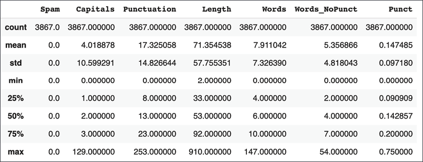
Figure 1.12: Statistics for regular messages after using POS tags

And then for spam messages:

train.loc[train['Spam']==1].describe()

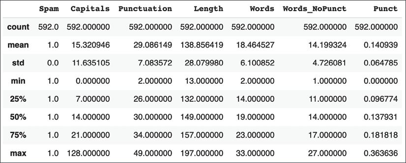
Figure 1.13: Statistics for spam messages after using POS tags

In general, word counts have been reduced even further after stop word removal. Further more, the new Punct feature computes the ratio of punctuation tokens in a message relative to the total tokens. Now we can build a model with this data.

Modeling data with POS tagging

Plugging these features into the model, the following results are obtained:

x_train = train[['Length', 'Punctuation', 'Capitals', 'Words_NoPunct', 'Punct']]
y_train = train[['Spam']]
x_test = test[['Length', 'Punctuation', 'Capitals' , 'Words_NoPunct', 'Punct']]
y_test = test[['Spam']]
model = make_model(input_dims=5)
# model = make_model(input_dims=3)
model.fit(x_train, y_train, epochs=10, batch_size=10)

Train on 4459 samples
Epoch 1/10
4459/4459 [==============================] - 1s 236us/sample - loss: 3.1958 - accuracy: 0.6028
Epoch 2/10
...
Epoch 10/10
4459/4459 [==============================] - 1s 139us/sample - loss: 0.1788 - accuracy: 0.9466

The accuracy shows a slight increase and is now up to 94.66%. Upon testing, it seems to hold:

model.evaluate(x_test, y_test)

1115/1115 [==============================] - 0s 91us/sample - loss: 0.2076 - accuracy: 0.9426
[0.20764057086989485, 0.9426009]

The final part of text normalization is stemming and lemmatization. Though we will not be building any features for the spam model using this, it can be quite useful in other cases.

Stemming and lemmatization

In certain languages, the same word can take a slightly different form depending on its usage. Consider the word depend itself. The following are all valid forms of the word depend: depends, depending, depended, dependent. Often, these variations are due to tenses. In some languages like Hindi, verbs may have different forms for different genders. Another case is derivatives of the same word such as sympathy, sympathetic, sympathize, and sympathizer. These variations can take different forms in other languages. In Russian, proper nouns take different forms based on usage. Suppose there is a document talking about London (Лондон). The phrase in London (в Лондоне) spells London differently than from London (из Лондона). These variations in the spelling of London can cause issues when matching some input to sections or words in a document.

When processing and tokenizing text to construct a vocabulary of words appearing in the corpora, the ability to identify the root word can reduce the size of the vocabulary while expanding the accuracy of matches. In the preceding Russian example, any form of the word London can be matched to any other form if all the forms are normalized to a common representation post-tokenization. This process of normalization is called stemming or lemmatization.

Stemming and lemmatization differ in their approach and sophistication but serve the same objective. Stemming is a simpler, heuristic rule-based approach that chops off the affixes of words. The most famous stemmer is called the Porter stemmer, published by Martin Porter in 1980. The official website is https://tartarus.org/martin/PorterStemmer/, where various versions of the algorithm implemented in various languages are linked.

This stemmer only works for English and has rules including removing s at the end of the words for plurals, and removing endings such as -ed or -ing. Consider the following sentence:

"Stemming is aimed at reducing vocabulary and aid understanding of morphological processes. This helps people understand the morphology of words and reduce size of corpus."

After stemming using Porter's algorithm, this sentence will be reduced to the following:

"Stem is aim at reduce vocabulari and aid understand of morpholog process . Thi help peopl understand the morpholog of word and reduc size of corpu ."

Note how different forms of morphology, understand, and reduce are all tokenized to the same form.

Lemmatization approaches this task in a more sophisticated manner, using vocabularies and morphological analysis of words. In the study of linguistics, a morpheme is a unit smaller than or equal to a word. When a morpheme is a word in itself, it is called a root or a free morpheme. Conversely, every word can be decomposed into one or more morphemes. The study of morphemes is called morphology. Using this morphological information, a word's root form can be returned post-tokenization. This base or dictionary form of the word is called a lemma, hence the process is called lemmatization. StanfordNLP includes lemmatization as part of processing.

Here is a simple piece of code to take the preceding sentences and parse them:

text = "Stemming is aimed at reducing vocabulary and aid understanding of morphological processes. This helps people understand the morphology of words and reduce size of corpus."
lemma = en(text)

After processing, we can iterate through the tokens to get the lemma of each word. This is shown in the following code fragment. The lemma of a word is exposed as the .lemma property of each word inside a token. For the sake of brevity of code, a simplifying assumption is made here that each token has only one word.

The POS for each word is also printed out to help us understand how the process was performed. Some key words in the following output are highlighted:

lemmas = ""
for sentence in lemma.sentences:
        for token in sentence.tokens:
            lemmas += token.words[0].lemma +"/" + \
                    token.words[0].upos + " "
        lemmas += "\n"
print(lemmas)

stem/NOUN be/AUX aim/VERB at/SCONJ reduce/VERB vocabulary/NOUN and/CCONJ aid/NOUN understanding/NOUN of/ADP morphological/ADJ process/NOUN ./PUNCT 
this/PRON help/VERB people/NOUN understand/VERB the/DET morphology/NOUN of/ADP word/NOUN and/CCONJ reduce/VERB size/NOUN of/ADP corpus/ADJ ./PUNCT

Compare this output to the output of the Porter stemmer earlier. One immediate thing to notice is that lemmas are actual words as opposed to fragments, as was the case with the Porter stemmer. In the case of reduce, the usage in both sentences is in the form of a verb, so the choice of lemma is consistent. Focus on the words understand and understanding in the preceding output. As the POS tag shows, it is used in two different forms. Consequently, it is not reduced to the same lemma. This is different from the Porter stemmer. The same behavior can be observed for morphology and morphological. This is a quite sophisticated behavior.

Now that text normalization is completed, we can begin the vectorization of text.