Missing Values

When there is no value (that is, a null value) recorded for a particular feature in a data point, we say that the data is missing. Having missing values in a real dataset is inevitable; no dataset is ever perfect. However, it is important to understand why the data is missing, and whether there is a factor that has affected the loss of data. Appreciating and recognizing this allows us to handle the remaining data in an appropriate manner. For example, if the data is missing randomly, then it's highly likely that the remaining data is still representative of the population. However, if the missing data is not random in nature and we assume that it is, it could bias our analysis and subsequent modeling.

Let's look at the common reasons (or mechanisms) for missing data:

• Missing Completely at Random (MCAR): Values in a dataset are said to be MCAR if there is no correlation whatsoever between the value missing and any other recorded variable or external parameter. This means that the remaining data is still representative of the population, though this is rarely the case and taking missing data to be completely random is usually an unrealistic assumption.

  For example, in a study that involves determining the reason for obesity among K12 children, MCAR is when the parents forgot to take their children to the clinic for the study.

• Missing at Random (MAR): If the case where the data is missing is related to the data that was recorded rather than the data that was not, then the data is said to be MAR. Since it's unfeasible to statistically verify whether data is MAR, we'd have to depend on whether it's a reasonable possibility.

  Using the K12 study, missing data in this case is due to parents moving to a different city, hence the children had to leave the study; missingness has nothing to do with the study itself.

• Missing Not at Random (MNAR): Data that is neither MAR nor MCAR is said to be MNAR. This is the case of a non-ignorable non-response, that is, the value of the variable that's missing is related to the reason it is missing.

  Continuing with the example of the case study, data would be MNAR if the parents were offended by the nature of the study and did not want their children to be bullied, so they withdrew their children from the study.

Finding Missing Values

So, now that we know why it's important to familiarize ourselves with the reasons behind why our data is missing, let's talk about how we can find these missing values in a dataset. For a pandas DataFrame, this is most commonly executed using the .isnull() method on a DataFrame to create a mask of the null values (that is, a DataFrame of Boolean values) indicating where the null values exist—a True value at any position indicates a null value, while a False value indicates the existence of a valid value at that position.

Note

The .isnull() method can be used interchangeably with the .isna() method for pandas DataFrames. Both these methods do exactly the same thing—the reason there are two methods to do the same thing is pandas DataFrames were originally based on R DataFrames, and hence have reproduced much of the syntax and ideas of the latter.

It may not be immediately obvious whether the missing data is random or not. Discovering the nature of missing values across features in a dataset is possible through two common visualization techniques:

• Nullity matrix: This is a data-dense display that lets us quickly visualize the patterns in data completion. It gives us a quick glance at how the null values within a feature (and across features) are distributed, how many there are, and how often they appear with other features.
• Nullity-correlation heatmap: This heatmap visually describes the nullity relationship (or a data completeness relationship) between each pair of features; that is, it measures how strongly the presence or absence of one variable affects the presence of another.

  Akin to regular correlation, nullity correlation values range from -1 to 1, the former indicating that one variable appears when the other definitely does not, and the latter indicating the simultaneous presence of both variables. A value of 0 implies that one variable having a null value has no effect on the other being null.

Exercise 2.02: Visualizing Missing Values

Let's analyze the nature of the missing values by first looking at the count and percentage of missing values for each feature, and then plotting a nullity matrix and correlation heatmap using the missingno library in Python. We will be using the same dataset from the previous exercises.

Please note that this exercise is a continuation of Exercise 2.01: Summarizing the Statistics of Our Dataset.

The following steps will help you complete this exercise to visualize the missing values in the dataset:

1. Calculate the count and percentage of missing values in each column and arrange these in decreasing order. We will use the .isnull() function on the DataFrame to get a mask. The count of null values in each column can then be found using the .sum() function over the DataFrame mask. Similarly, the fraction of null values can be found using .mean() over the DataFrame mask and multiplied by 100 to convert it to a percentage.

   Then, we combine the total and percentage of null values into a single DataFrame using the pd.concat() function, and subsequently sort the rows by percentage of missing values and print the DataFrame:

   mask = data.isnull()
   total = mask.sum()
   percent = 100*mask.mean()
   missing_data = pd.concat([total, percent], axis=1,join='outer', \
                            keys=['count_missing', 'perc_missing'])
   missing_data.sort_values(by='perc_missing', ascending=False, \
                            inplace=True)
   missing_data

   The output will be as follows:

   

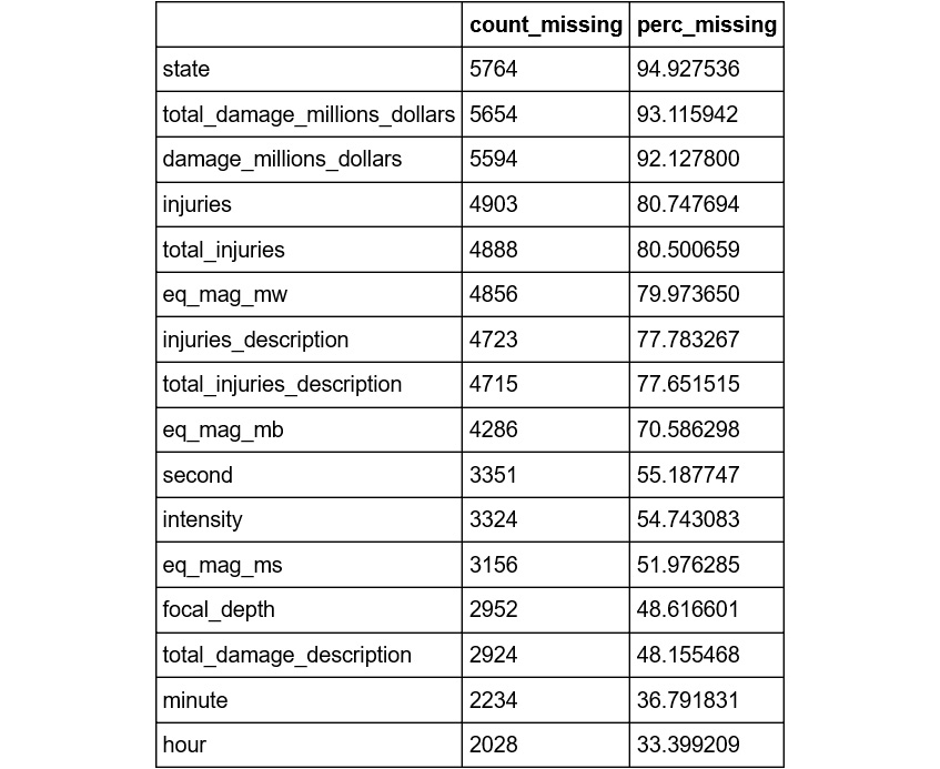
   Figure 2.5: The count and percentage of missing values in each column

   Here, we can see that the state, total_damage_millions_dollars, and damage_millions_dollars columns have over 90% missing values, which means that data for fewer than 10% of the data points in the dataset are available for these columns. On the other hand, year, flag_tsunami, country, and region_code have no missing values.

2. Plot the nullity matrix. First, we find the list of columns that have any null values in them using the .any() function on the DataFrame mask from the previous step. Then, we use the missingno library to plot the nullity matrix for a random sample of 500 data points from our dataset, for only those columns that have missing values:

   nullable_columns = data.columns[mask.any()].tolist()
   msno.matrix(data[nullable_columns].sample(500))
   plt.show()

   The output will be as follows:

   

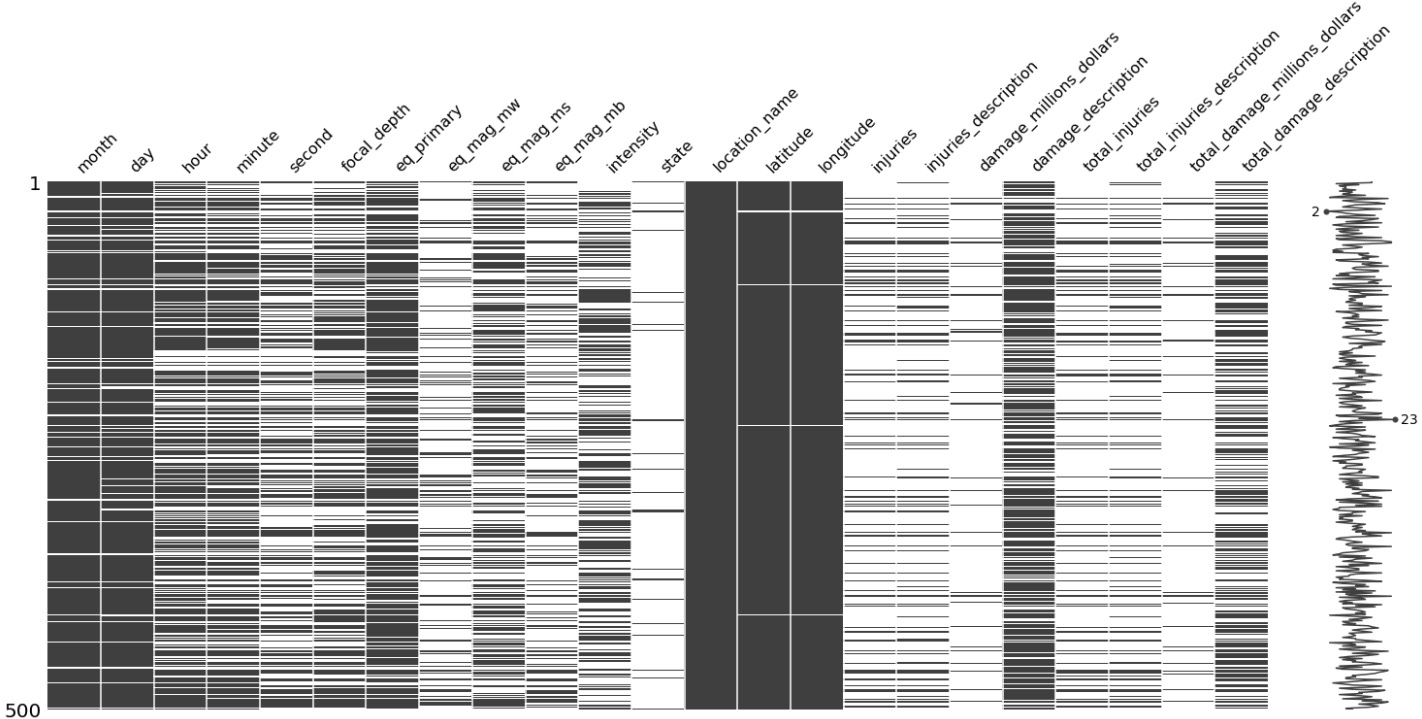
   Figure 2.6: The nullity matrix

   Here, black lines represent non-nullity while the white lines indicate the presence of a null value in that column. At a glance, location_name appears to be completely populated (we know from the previous step that there is, in fact, only one missing value in this column), while latitude and longitude seem mostly complete, but spottier.

   The spark line on the right summarizes the general shape of the data completeness and points out the rows with the maximum and minimum nullity in the dataset. Note that this is only for the sample of 500 points.

3. Plot the nullity correlation heatmap. We will plot the nullity correlation heatmap using the missingno library for our dataset, for only those columns that have missing values:

   msno.heatmap(data[nullable_columns], figsize=(18,18))
   plt.show()

   The output will be as follows:

   

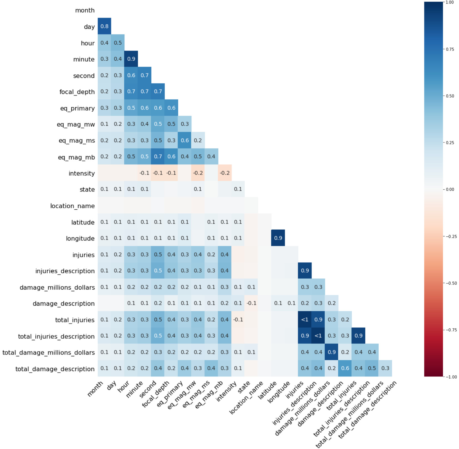
Figure 2.7: The nullity correlation heatmap

Here, we can also see some boxes labeled <1: this just means that the correlation values in those cases are all close to 1.0, but still not quite perfectly so. We can see a value of <1 between injuries and total_injuries, which means that the missing values in each category are correlated. We would need to dig deeper to understand whether the missing values are correlated because they are based upon the same or similar information, or for some other reason.

Note

To access the source code for this specific section, please refer to https://packt.live/2YSXq3k.

You can also run this example online at https://packt.live/2Yn3Us7. You must execute the entire Notebook in order to get the desired result.

Imputation Strategies for Missing Values

There are multiple ways of dealing with missing values in a column. The simplest way is to simply delete rows having missing values; however, this can result in the loss of valuable information from other columns. Another option is to impute the data, that is, replace the missing values with a valid value inferred from the known part of the data. The common ways in which this can be done are listed here:

• Create a new value that is distinct from the other values to replace the missing values in the column so as to differentiate those rows altogether. Then, use a non-linear machine learning algorithm (such as ensemble models or support vectors) that can separate the values out.
• Use an appropriate central value from the column (mean, median, or mode) to replace the missing values.
• Use a model (such as a K-nearest neighbors or a Gaussian mixture model) to learn the best value with which to replace the missing values.

Python has a few functions that are useful for replacing null values in a column with a static value. One way to do this is to use the inherent pandas .fillna(0) function: there is no ambiguity in imputation here—the static value with which to substitute the null data point in the column is the argument being passed to the function (the value in the brackets).

However, if the number of null values in a column is significant and it's not immediately obvious what the appropriate central value is that can be used to replace each null value, then we can either delete the rows having null values or delete the column altogether from the modeling perspective, as it may not add any significant value. This can be done by using the .dropna() function on the DataFrame. The parameters that can be passed to the function are as follows:

• axis: This defines whether to drop rows or columns, which is determined by assigning the parameter a value of 0 or 1, respectively.
• how: A value of all or any can be assigned to this parameter to indicate whether the row/column should contain all null values to drop the column, or whether to drop the column if there is at least one null value.
• thresh: This defines the minimum number of null values the row/column should have in order to be dropped.

Additionally, if an appropriate replacement for a null value for a categorical feature cannot be determined, a possible alternative to deleting the column is to create a new category in the feature that can represent the null values.

Note

If it is immediately obvious how a null value for a column can be replaced from an intuitive understanding or domain knowledge, then we can replace the value on the spot. Keep in mind that any such data changes should be made in your code and never directly on the raw data. One reason for this is that it allows the strategy to be updated easily in the future. Another reason is that it makes it visible to others who may later be reviewing the work where changes were made. Directly changing raw data can lead to data versioning problems and make it impossible for others to reproduce your work. In many cases, inferences become more obvious at later stages in the exploration process. In these cases, we can substitute null values as and when we find an appropriate way to do so.

Exercise 2.03: Performing Imputation Using Pandas

Let's look at missing values and replace them with zeros in time-based (continuous) features having at least one null value (month, day, hour, minute, and second). We do this because, for cases where we do not have recorded values, it would be safe to assume that the events take place at the beginning of the time duration. This exercise is a continuation of Exercise 2.02: Visualizing Missing Values:

1. Create a list containing the names of the columns whose values we want to impute:

   time_features = ['month', 'day', 'hour', 'minute', 'second']

2. Impute the null values using .fillna(). We will replace the missing values in these columns with 0 using the inherent pandas .fillna() function and pass 0 as an argument to the function:

   data[time_features] = data[time_features].fillna(0)

3. Use the .info() function to view null value counts for the imputed columns:

   data[time_features].info()

   The output will be as follows:

   

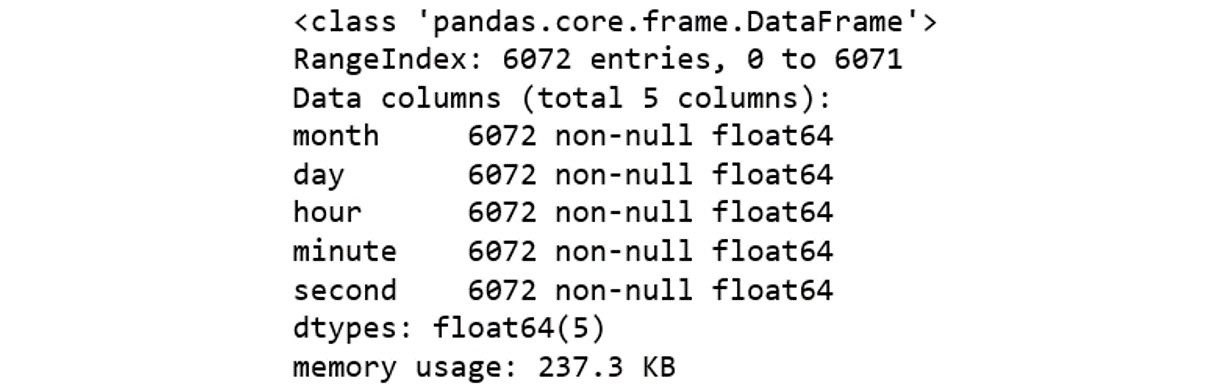
Figure 2.8: Null value counts

As we can now see, all values for our features in the DataFrame are now non-null.

Note

To access the source code for this specific section, please refer to https://packt.live/2V9nMx3.

You can also run this example online at https://packt.live/2BqoZZM. You must execute the entire Notebook in order to get the desired result.

Exercise 2.04: Performing Imputation Using Scikit-Learn

In this exercise, you will replace the null values in the description-related categorical features using scikit-learn's SimpleImputer class. In Exercise 2.02: Visualizing Missing Values, we saw that almost all of these features comprised more than 50% of null values in the data. Replacing these null values with a central value might bias any model we try to build using the features, deeming them irrelevant. Let's instead replace the null values with a separate category, having the value NA. This exercise is a continuation of Exercise 2.02: Visualizing Missing Values:

1. Create a list containing the names of the columns whose values we want to impute:

   description_features = ['injuries_description', \
                           'damage_description', \
                           'total_injuries_description', \
                           'total_damage_description']

2. Create an object of the SimpleImputer class. Here, we first create an imp object of the SimpleImputer class and initialize it with parameters that represent how we want to impute the data. The parameters we will pass to initialize the object are as follows:

   missing_values: This is the placeholder for the missing values, that is, all occurrences of the values in the missing_values parameter will be imputed.

   strategy: This is the imputation strategy, which can be one of mean, median, most_frequent (that is, the mode), or constant. While the first three can only be used with numeric data and will replace missing values using the specified central value along each column, the last one will replace missing values with a constant as per the fill_value parameter.

   fill_value: This specifies the value with which to replace all occurrences of missing_values. If left to the default, the imputed value will be 0 when imputing numerical data and the missing_value string for strings or object data types:

   imp = SimpleImputer(missing_values=np.nan, \
                       strategy='constant', \
                       fill_value='NA')

3. Perform the imputation. We will use imp.fit_transform() to actually perform the imputation. It takes the DataFrame with null values as input and returns the imputed DataFrame:

   data[description_features] = \
   imp.fit_transform(data[description_features])

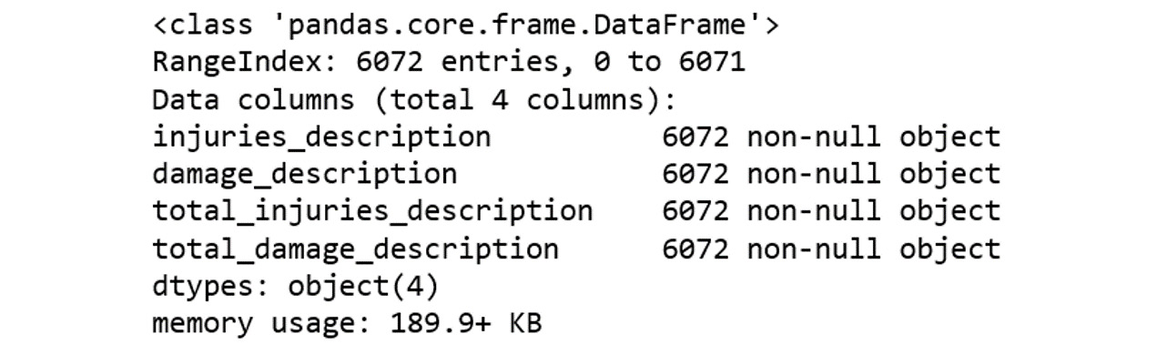
4. Use the .info() function to view null value counts for the imputed columns:

   data[description_features].info()

   The output will be as follows:

   

Figure 2.9: The null value counts

Note

To access the source code for this specific section, please refer to https://packt.live/3ervLgk.

You can also run this example online at https://packt.live/3doEX3G. You must execute the entire Notebook in order to get the desired result.

In the last two exercises, we looked at two ways to use pandas and scikit-learn methods to impute missing values. These methods are very basic methods we can use if we have little or no information about the underlying data. Next, we'll look at more advanced techniques we can use to fill in missing data.

Exercise 2.05: Performing Imputation Using Inferred Values

Let's replace the null values in the continuous damage_millions_dollars feature with information from the categorical damage_description feature. Although we may not know the exact dollar amount that was incurred, the categorical feature gives us information on the range of the amount that was incurred due to damage from the earthquake. This exercise is a continuation of Exercise 2.04: Performing Imputation Using scikit-learn:

1. Find how many rows have null damage_millions_dollars values, and how many of those have non-null damage_description values:

   print(data[pd.isnull(data.damage_millions_dollars)].shape[0])
   print(data[pd.isnull(data.damage_millions_dollars) \
              & (data.damage_description != 'NA')].shape[0])

   The output will be as follows:

   5594
   3849

   As we can see, 3,849 of 5,594 null values can be easily substituted with the help of another variable. For example, we know that all variables having column names ending with _description are a descriptor field containing estimates for data that may not be available in the original numerical column. For deaths, injuries, and total_injuries, the corresponding categorical values represent the following:

   0 = None

   1 = Few (~1 to 50 deaths)

   2 = Some (~51 to 100 deaths)

   3 = Many (~101 to 1,000 deaths)

   4 = Very Many (~1,001 or more deaths)

   As regards damage_millions_dollars, the corresponding categorical values represent the following:

   0 = None

   1 = Limited (roughly corresponding to less than 1 million dollars)

   2 = Moderate (~1 to 5 million dollars)

   3 = Severe (~>5 to 24 million dollars)

   4 = Extreme (~25 million dollars or more)

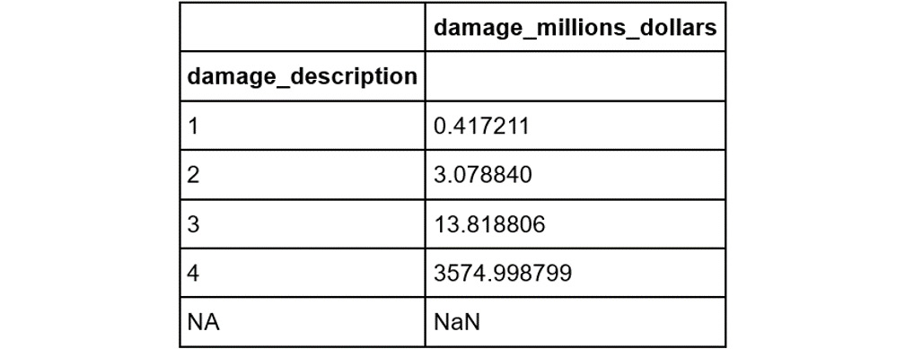
2. Find the mean damage_millions_dollars value for each category. Since each of the categories in damage_description represents a range of values, we find the mean damage_millions_dollars value for each category from the non-null values already available. These provide a reasonable estimate for the most likely value for that category:

   category_means = data[['damage_description', \
                          'damage_millions_dollars']]\
                          .groupby('damage_description').mean()
   category_means

   The output will be as follows:

   

   Figure 2.10: The mean damage_millions_dollars value for each category

   Note that the first three values make intuitive sense given the preceding definitions: 0.42 is between 0 and 1, 3.1 is between 1 and 5, and 13.8 is between 5 and 24. The last category is defined as 25 million or more; it transpires that the mean of these extreme cases is very high (3,575!).

3. Store the mean values as a dictionary. In this step, we will convert the DataFrame containing the mean values to a dictionary (a Python dict object), so that accessing them is convenient.

   Additionally, since the value for the newly created NA category (the imputed value in the previous exercise) was NaN, and the value for the 0 category was absent (no rows had damage_description equal to 0 in the dataset), we explicitly added these values to the dictionary as well:

   replacement_values = category_means\
                        .damage_millions_dollars.to_dict()
   replacement_values['NA'] = -1
   replacement_values['0'] = 0
   replacement_values

   The output will be as follows:

   

   Figure 2.11: The dictionary of mean values

4. Create a series of replacement values. For each value in the damage_description column, we map the categorical value onto the mean value using the map function. The .map() function is used to map the keys in the column to the corresponding values for each element from the replacement_values dictionary:

   imputed_values = data.damage_description.map(replacement_values)

5. Replace null values in the column. We do this by using np.where as a ternary operator: the first argument is the mask, the second is the series from which to take the value if the mask is positive, and the third is the series from which to take the value if the mask is negative.

   This ensures that the array returned by np.where only replaces the null values in damage_millions_dollars with values from the imputed_values series:

   data['damage_millions_dollars'] = \
   np.where(data.damage_millions_dollars.isnull(), \
   data.damage_description.map(replacement_values), \
   data.damage_millions_dollars)

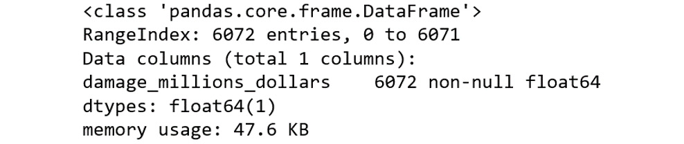
6. Use the .info() function to view null value counts for the imputed columns:

   data[['damage_millions_dollars']].info()

   The output will be as follows:

   

Figure 2.12: The null value counts

We can see that, after replacement, there are no null values in the damage_millions_dollars column.

Note

To access the source code for this specific section, please refer to https://packt.live/3fMRqQo.

You can also run this example online at https://packt.live/2YkBgYC. You must execute the entire Notebook in order to get the desired result.

In this section, we have looked at replacing missing values in more than one way. In one case, we replaced values with zeros; in another case, we looked at more information about the dataset to reason that we could replace missing values with a combination of information from a descriptive field and the means of values we did have. These sorts of decisions and steps are extremely common when working with real data. We also noted that, occasionally, when we have sufficient data and the instances with missing values are few, we can just drop them. In the following activity, we'll use a different dataset for you to practice and reinforce these methods.

Activity 2.01: Summary Statistics and Missing Values

In this activity, we'll revise some of the summary statistics and missing value exploration we have looked at thus far in this chapter. We will be using a new dataset, House Prices: Advanced Regression Techniques, available on Kaggle.

Note

The original dataset is available at https://www.kaggle.com/c/house-prices-advanced-regression-techniques/data or on our GitHub repository at https://packt.live/2TjU9aj.

While the Earthquakes dataset used in the exercises is aimed at solving a classification problem (when the target variable has only discrete values), the dataset we will use in the activities will be aimed at solving a regression problem (when the target variable takes on a range of continuous values). We will use pandas functions to generate summary statistics and visualize missing values using a nullity matrix and nullity correlation heatmap.

The steps to be performed are as follows:

1. Read the data (house_prices.csv).
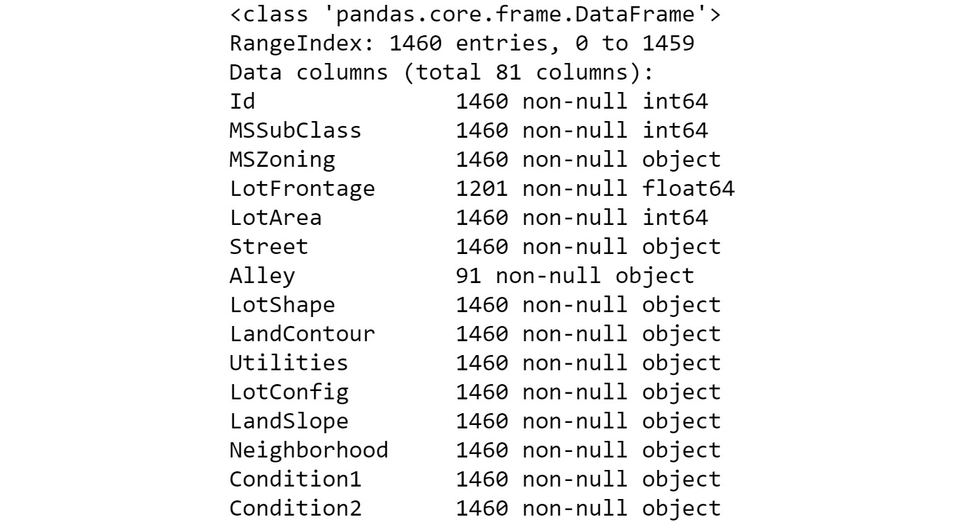
2. Use pandas' .info() and .describe() methods to view the summary statistics of the dataset.

   The output of the info() method will be as follows:

   

   Figure 2.13: The output of the info() method (abbreviated)

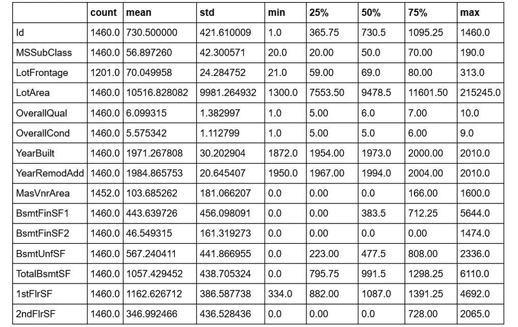
   The output of the describe() method will be as follows:

   

   Figure 2.14: The output of the describe() method (abbreviated)

   Note

   The outputs of the info() and describe() methods have been truncated for presentation purposes. You can find the outputs in their entirety here: https://packt.live/2TjZSgi

3. Find the total count and total percentage of missing values in each column of the DataFrame and display them for columns having at least one null value, in descending order of missing percentages.
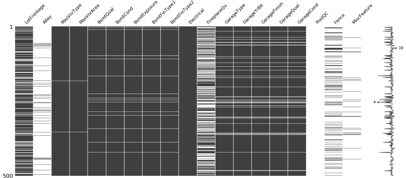
4. Plot the nullity matrix and nullity correlation heatmap.

   The nullity matrix will be as follows:

   

   Figure 2.15: Nullity matrix

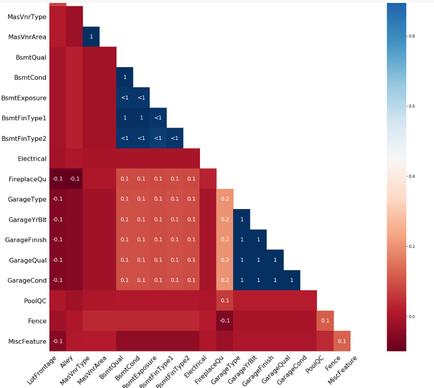
   The nullity correlation heatmap will be as follows:

   

   Figure 2.16: Nullity correlation heatmap

5. Delete the columns having more than 80% of their values missing.
6. Replace null values in the FireplaceQu column with NA values.

   Note

   The solution for this activity can be found via this link.

You should now be comfortable using the approaches we've learned to investigate missing values in any type of tabular data.