Setting up a virtual environment

This book was written using Python 3.7.3, but the code should work for Python 3.7.1+, which is available on all major operating systems. In this section, we will go over how to set up the virtual environment in order to follow along with this book. If Python isn't already installed on your computer, read through the following sections on virtual environments first, and then decide whether to install Anaconda, since it will also install Python. To install Python without Anaconda, download it from https://www.python.org/downloads/, and then follow the venv section instead of the conda section.

Important note

To check whether Python is already installed, run where python3 from the command line on Windows or which python3 from the command line on Linux/macOS. If this returns nothing, try running it with just python (instead of python3). If Python is installed, check the version by running python3 --version. Note that if python3 works, then you should use that throughout the book (and conversely, use python if python3 doesn't work).

Virtual environments

Most of the time, when we want to install software on our computer, we simply download it, but the nature of programming languages where packages are constantly being updated and rely on specific versions of others means this can cause issues. We could be working on a project one day where we need a certain version of a Python package (say 0.9.1), but the next day be working on an analysis where we need the most recent version of that same package to access some newer functionality (1.1.0). Sounds like there wouldn't be an issue, right? Well, what happens if this update causes a breaking change to the first project or another package in our project that relies on this one? This is a common enough problem that a solution already exists to prevent this from being an issue: virtual environments.

A virtual environment allows us to create separate environments for each of our projects. Each of our environments will only have the packages that it needs installed. This makes it easy to share our environment with others, have multiple versions of the same package installed on our machine for different projects without interfering with each other, and avoid unexpected side effects from installing packages that update or have dependencies on others. It's good practice to make a dedicated virtual environment for any projects we work on.

We will discuss two common ways to achieve this setup, and you can decide which fits best. Note that all the code in this section will be executed on the command line.

venv

Python 3 comes with the venv module, which will create a virtual environment in the location of our choice. The process of setting up and using a development environment is as follows (after Python is installed):

1. Create a folder for the project.
2. Use venv to create an environment in this folder.
3. Activate the environment.
4. Install Python packages in the environment with pip.
5. Deactivate the environment when finished.

In practice, we will create environments for each project we work on, so our first step will be to create a directory for all of our project files. For this, we can use the mkdir command. Once this has been created, we will change our current directory to the newly created one using the cd command. Since we already obtained the project files (from the instructions in the Chapter materials section), the following is for reference only. To make a new directory and move to that directory, we can use the following command:

$ mkdir my_project && cd my_project

Tip

cd <path> changes the current directory to the path specified in <path>, which can be an absolute (full) path or relative (how to get there from the current directory) path.

Before moving on, use cd to navigate to the directory containing this book's repository. Note that the path will depend on where it was cloned/downloaded:

$ cd path/to/Hands-On-Data-Analysis-with-Pandas-2nd-edition

Since there are slight differences in operating systems for the remaining steps, we will go over Windows and Linux/macOS separately. Note that if you have both Python 2 and Python 3, make sure you use python3 and not python in the following commands.

Windows

To create our environment for this book, we will use the venv module from the standard library. Note that we must provide a name for our environment (book_env). Remember, if your Windows setup has python associated with Python 3, then use python instead of python3 in the following command:

C:\...> python3 -m venv book_env

Now, we have a folder for our virtual environment named book_env inside the repository folder that we cloned/downloaded earlier. In order to use the environment, we need to activate it:

C:\...> %cd%\book_env\Scripts\activate.bat

Tip

Windows replaces %cd% with the path to the current directory. This saves us from having to type the full path up to the book_env part.

Note that after we activate the virtual environment, we can see (book_env) in front of our prompt on the command line; this lets us know we are in the environment:

(book_env) C:\...> 

When we are finished using the environment, we simply deactivate it:

(book_env) C:\...> deactivate

Any packages that are installed in the environment don't exist outside the environment. Note that we no longer have (book_env) in front of our prompt on the command line. You can read more about venv in the Python documentation at https://docs.python.org/3/library/venv.html.

Now that the virtual environment is created, activate it and then head to the Installing the required Python packages section for the next step.

Linux/macOS

To create our environment for this book, we will use the venv module from the standard library. Note that we must provide a name for our environment (book_env):

$ python3 -m venv book_env

Now, we have a folder for our virtual environment named book_env inside of the repository folder we cloned/downloaded earlier. In order to use the environment, we need to activate it:

$ source book_env/bin/activate

Note that after we activate the virtual environment, we can see (book_env) in front of our prompt on the command line; this lets us know we are in the environment:

(book_env) $

When we are finished using the environment, we simply deactivate it:

(book_env) $ deactivate

Any packages that are installed in the environment don't exist outside the environment. Note that we no longer have (book_env) in front of our prompt on the command line. You can read more about venv in the Python documentation at https://docs.python.org/3/library/venv.html.

Now that the virtual environment is created, activate it and then head to the Installing the required Python packages section for the next step.

conda

Anaconda provides a way to set up a Python environment specifically for data science. It includes some of the packages we will use in this book, along with several others that may be necessary for tasks that aren't covered in this book (and also deals with dependencies outside of Python that might be tricky to install otherwise). Anaconda uses conda as the environment and package manager instead of pip, although packages can still be installed with pip (as long as the pip installed by Anaconda is called). Note that some packages may not be available with conda, in which case we will have to use pip. Consult this page in the conda documentation for a comparison of commands used with conda, pip, and venv: https://conda.io/projects/conda/en/latest/commands.html#conda-vs-pip-vs-virtualenv-commands.

Important note

Be warned that Anaconda is a very large install (although the Miniconda version is much lighter). Those who use Python for purposes aside from data science may prefer the venv method we discussed earlier in order to have more control over what gets installed.

Anaconda can also be packaged with the Spyder integrated development environment (IDE) and Jupyter Notebooks, which we will discuss later. Note that we can use Jupyter with the venv option as well.

You can read more about Anaconda and how to install it at the following pages in their official documentation:

• Windows: https://docs.anaconda.com/anaconda/install/windows/
• macOS: https://docs.anaconda.com/anaconda/install/mac-os/
• Linux: https://docs.anaconda.com/anaconda/install/linux/
• User guide: https://docs.anaconda.com/anaconda/user-guide/

Once you have installed either Anaconda or Miniconda, confirm that it is properly installed by running conda -V on the command line to display the version. Note that on Windows, all conda commands need to be run in Anaconda Prompt (as opposed to Command Prompt).

To create a new conda environment for this book, called book_env, run the following:

(base) $ conda create --name book_env

Running conda env list will show all the conda environments on the system, which will now include book_env. The current active environment will have an asterisk (*) next to it—by default, base will be active until we activate another environment:

(base) $ conda env list
# conda environments:
#
base                  *  /miniconda3
book_env                 /miniconda3/envs/book_env

To activate the book_env environment, we run the following command:

(base) $ conda activate book_env

Note that after we activate the virtual environment, we can see (book_env) in front of our prompt on the command line; this lets us know we are in the environment:

(book_env) $

When we are finished using the environment, we deactivate it:

(book_env) $ conda deactivate

Any packages that are installed in the environment don't exist outside the environment. Note that we no longer have (book_env) in front of our prompt on the command line. You can read more about how to use conda to manage virtual environments at https://www.freecodecamp.org/news/why-you-need-python-environments-and-how-to-manage-them-with-conda-85f155f4353c/.

In the next section, we will install the Python packages required for following along with this book, so be sure to activate the virtual environment now.

Installing the required Python packages

We can do a lot with the Python standard library; however, we will often find the need to install and use an outside package to extend functionality. The requirements.txt file in the repository contains all the packages we need to install to work through this book. It will be in our current directory, but it can also be found at https://github.com/stefmolin/Hands-On-Data-Analysis-with-Pandas-2nd-edition/blob/master/requirements.txt. This file can be used to install a bunch of packages at once with the -r flag in the call to pip3 install and has the advantage of being easy to share.

Before installing anything, be sure to activate the virtual environment that you created with either venv or conda. Be advised that if the environment is not activated before running the following command, the packages will be installed outside the environment:

(book_env) $ pip3 install -r requirements.txt

Tip

If you encounter any issues, report them at https://github.com/stefmolin/Hands-On-Data-Analysis-with-Pandas-2nd-edition/issues.

Why pandas?

When it comes to data science in Python, the pandas library is pretty much ubiquitous. It is built on top of the NumPy library, which allows us to perform mathematical operations on arrays of single-type data efficiently. Pandas expands this to dataframes, which can be thought of as tables of data. We will get a more formal introduction to dataframes in Chapter 2, Working with Pandas DataFrames.

Aside from efficient operations, pandas also provides wrappers around the matplotlib plotting library, making it very easy to create a variety of plots without needing to write many lines of matplotlib code. We can always tweak our plots using matplotlib, but for quickly visualizing our data, we only need one line of code in pandas. We will explore this functionality in Chapter 5, Visualizing Data with Pandas and Matplotlib, and Chapter 6, Plotting with Seaborn and Customization Techniques.

Important note

Wrapper functions wrap around code from another library, obscuring some of its complexity and leaving us with a simpler interface for repeating that functionality. This is a core principle of object-oriented programming (OOP) called abstraction, which reduces complexity and the duplication of code. We will create our own wrapper functions throughout this book.

In addition to pandas, this book makes use of Jupyter Notebooks. While you are free to choose not to use them, it's important to be familiar with Jupyter Notebooks as they are very common in the data world. As an introduction, we will use a Jupyter Notebook to validate our setup in the next section.

Jupyter Notebooks

Each chapter of this book includes Jupyter Notebooks for following along. Jupyter Notebooks are omnipresent in Python data science because they make it very easy to write and test code in more of a discovery environment compared to writing a program. We can execute one block of code at a time and have the results printed to the notebook, directly beneath the code that generated it. In addition, we can use Markdown to add text explanations to our work. Jupyter Notebooks can be easily packaged up and shared; they can be pushed to GitHub (where they will be rendered), converted into HTML or PDF, sent to someone else, or presented.

Launching JupyterLab

JupyterLab is an IDE that allows us to create Jupyter Notebooks and Python scripts, interact with the terminal, create text documents, reference documentation, and much more from a clean web interface on our local machine. There are lots of keyboard shortcuts to master before really becoming a power user, but the interface is pretty intuitive. When we created our environment, we installed everything we needed to run JupyterLab, so let's take a quick tour of the IDE and make sure that our environment is set up properly. First, we activate our environment, and then we launch JupyterLab:

(book_env) $ jupyter lab

This will then launch a window in the default browser with JupyterLab. We will be greeted with the Launcher tab and the File Browser pane to the left:

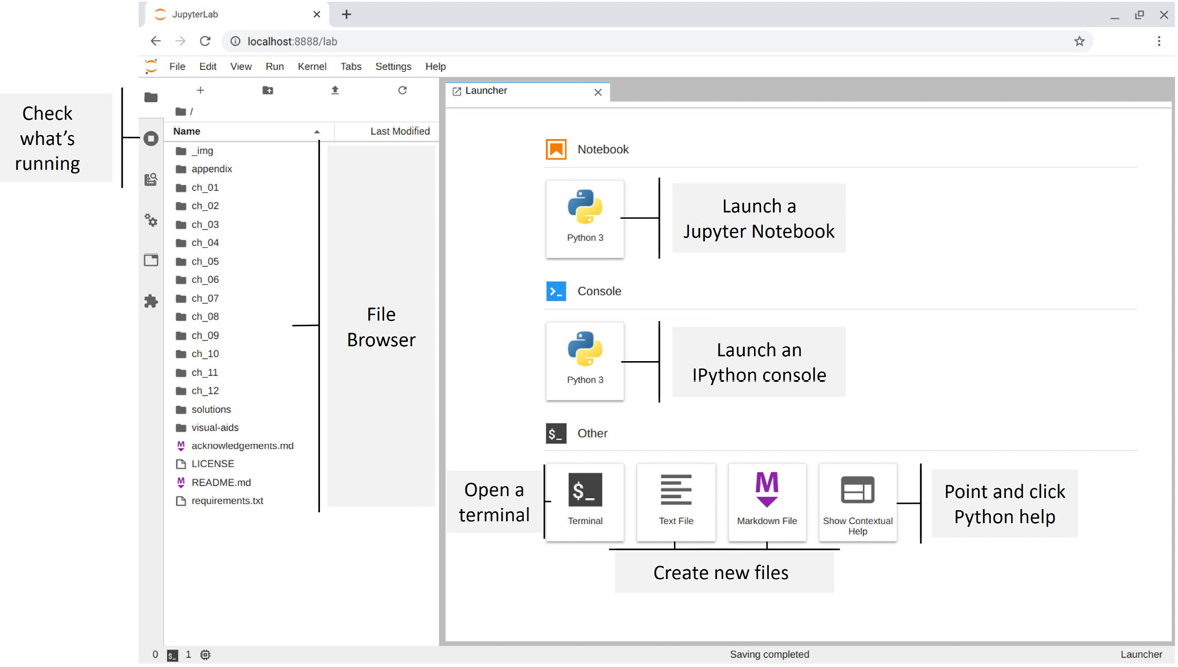
Figure 1.18 – Launching JupyterLab

Using the File Browser pane, double-click on the ch_01 folder, which contains the Jupyter Notebook that we will use to validate our setup.

Validating the virtual environment

Open the checking_your_setup.ipynb notebook in the ch_01 folder, as shown in the following screenshot:

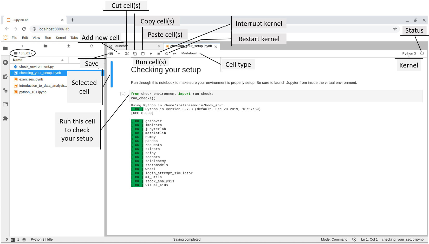
Figure 1.19 – Validating the virtual environment setup

Important note

The kernel is the process that runs and introspects our code in a Jupyter Notebook. Note that we aren't limited to running Python—we can run kernels for R, Julia, Scala, and other languages as well. By default, we will be running Python using the IPython kernel. We will learn a little more about IPython throughout the book.

Click on the code cell indicated in the previous screenshot and run it by clicking the play (▶) button. If everything shows up in green, the environment is all set up. However, if this isn't the case, run the following command from the virtual environment to create a special kernel with the book_env virtual environment for use with Jupyter:

(book_env) $ ipython kernel install --user --name=book_env

This adds an additional option in the Launcher tab, and we can now switch to the book_env kernel from a Jupyter Notebook as well:

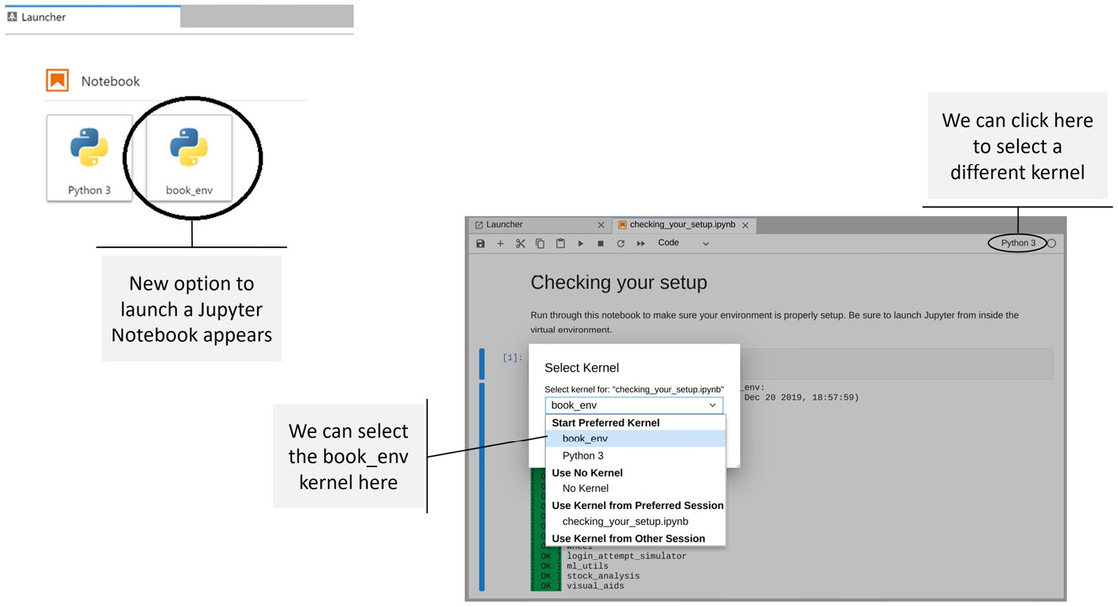
Figure 1.20 – Selecting a different kernel

It's important to note that Jupyter Notebooks will retain the values we assign to variables while the kernel is running, and the results in the Out[#] cells will be saved when we save the file. Closing the file doesn't stop the kernel and neither does closing the JupyterLab tab in the browser.

Closing JupyterLab

Closing the browser with JupyterLab in it doesn't stop JupyterLab or the kernels it is running (we also won't get the command-line interface back). To shut down JupyterLab entirely, we need to hit Ctrl + C (which is a keyboard interrupt signal that lets JupyterLab know we want to shut it down) a couple of times in the terminal until we get the prompt back:

...
[I 17:36:53.166 LabApp] Interrupted...
[I 17:36:53.168 LabApp] Shutting down 1 kernel
[I 17:36:53.770 LabApp] Kernel shutdown: a38e1[...]b44f
(book_env) $

For more information about Jupyter, including a tutorial, check out http://jupyter.org/. Learn more about JupyterLab at https://jupyterlab.readthedocs.io/en/stable/.