Book Image

Bayesian Analysis with Python - Third Edition

By : Osvaldo Martin
Book Image

Bayesian Analysis with Python - Third Edition

By: Osvaldo Martin

Overview of this book

The third edition of Bayesian Analysis with Python serves as an introduction to the main concepts of applied Bayesian modeling using PyMC, a state-of-the-art probabilistic programming library, and other libraries that support and facilitate modeling like ArviZ, for exploratory analysis of Bayesian models; Bambi, for flexible and easy hierarchical linear modeling; PreliZ, for prior elicitation; PyMC-BART, for flexible non-parametric regression; and Kulprit, for variable selection. In this updated edition, a brief and conceptual introduction to probability theory enhances your learning journey by introducing new topics like Bayesian additive regression trees (BART), featuring updated examples. Refined explanations, informed by feedback and experience from previous editions, underscore the book's emphasis on Bayesian statistics. You will explore various models, including hierarchical models, generalized linear models for regression and classification, mixture models, Gaussian processes, and BART, using synthetic and real datasets. By the end of this book, you will possess a functional understanding of probabilistic modeling, enabling you to design and implement Bayesian models for your data science challenges. You'll be well-prepared to delve into more advanced material or specialized statistical modeling if the need arises.
Table of Contents (15 chapters)
Preface
12
Bibliography
13
Other Books You May Enjoy
14
Index

6.4 Splines

A general way to write very flexible models is to apply functions Bm to Xm and then multiply them by coefficients βm:

μ = 𝛽0 + 𝛽1B1 (X1) + 𝛽2B2(X2 )+ ⋅⋅⋅+ 𝛽mBm (Xm )

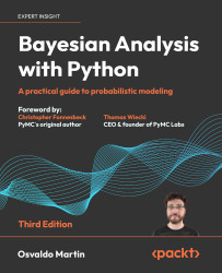
We are free to pick Bm as we wish; for instance, we can pick polynomials. But we can also pick other functions. A popular choice is to use B-splines; we are not going to discuss their definition, but we can think of them as a way to create smooth curves in such a way that we get flexibility, as with polynomials, but less prone to overfitting. We achieve this by using piecewise polynomials, that is, polynomials that are restricted to affect only a portion of the data. Figure 6.6 shows three examples of piecewise polynomials of increasing degrees. The dotted vertical lines show the ”knots,” which are the points used to restrict the regions, the dashed gray line represents the function we want to approximate, and the black lines are the piecewise polynomials.

PIC

Figure 6.6: Piecewise polynomials of increasing degrees

Figure 6.7 shows...