Traditionally, we could use the base R summary() function to identify some basic statistics. Now, and recently I might add, I like to use the package sjmisc and its descr() function. It produces a more readable output, and you can assign that output to a dataframe. What works well is to create that dataframe, save it as a .csv, and explore it at your leisure. It automatically selects numeric features only. It also fits well with tidyverse so that you can incorporate dplyr functions such as group_by() and filter(). Here's an example in our case where we examine the descriptive stats for the infantry of the Confederate Army. The output will consist of the following:

gettysburg %>%
  dplyr::filter(army == "Confederate" & type == "Infantry") %>%
  sjmisc::descr() -> descr_stats

readr::write_csv(descr_stats, 'descr_stats.csv')

The following is abbreviated output from the preceding code saved to a spreadsheet:

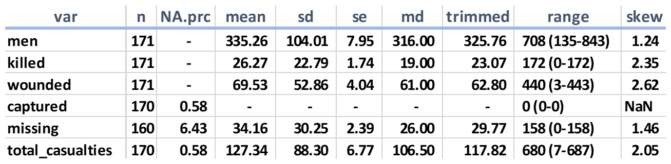
In this one table, we can discern some rather interesting tidbits. In particular is the percent of missing values per feature. If you modify the precious code to examine the Union Army, you'll find that there're no missing values. The reason the usurpers from the South had missing values is based on a couple of factors; either shoddy staff work in compiling the numbers on July 3^rd or the records were lost over the years. Note that, for the number of men captured, if you remove the missing value, all other values are zero, so we could just replace the missing value with it. The Rebels did not report troops as captured, but rather as missing, in contrast with the Union.

Once you feel comfortable with the descriptive statistics, move on to exploring the categorical features in the next section.

When it comes to an understanding of your categorical variables, there're many different ways to go about it. We can easily use the base R table() function on a feature. If you just want to see how many distinct levels are in a feature, then dplyr works well. In this example, we examine type, which has three unique levels:

dplyr::count(gettysburg, dplyr::n_distinct(type))

The output of the preceding code is as follows:

# A tibble: 1 x 2
     `dplyr::n_distinct(type)`        n
                                            <int> <int>
                                                     3    587

Let's now look at a way to explore all of the categorical features utilizing tidyverse principles. Doing it this way always allows you to save the tibble and examine the results in depth as needed. Here is a way of putting all categorical features into a separate tibble:

gettysburg_cat <-
  gettysburg[, sapply(gettysburg, class) == 'character']

Using dplyr, you can now summarize all of the features and the number of distinct levels in each:

gettysburg_cat %>%
  dplyr::summarise_all(dplyr::funs(dplyr::n_distinct(.)))

The output of the preceding code is as follows:

# A tibble: 1 x 9
   type  state regiment_or_battery brigade division corps  army july1_Commander  Cdr_casualty
 <int> <int>                                  <int>      <int>      <int> <int> <int>                            <int>                  <int>
          3       30                                      275           124            38        14          2                                586                           6

Notice that there're 586 distinct values to july1_Commander. This means that two of the unit Commanders have the same rank and last name. We can also surmise that this feature will be of no value to any further analysis, but we'll deal with that issue in a couple of sections ahead.

Suppose we're interested in the number of observations for each of the levels for the Cdr_casualty feature. Yes, we could use table(), but how about producing the output as a tibble as discussed before? Give this code a try:

gettysburg_cat %>% 
  dplyr::group_by(Cdr_casualty) %>%
  dplyr::summarize(num_rows = n())

The output of the preceding code is as follows:

# A tibble: 6 x 2
 Cdr_casualty                    num_rows
    <chr>                           <int>
 1 captured                            6
 2 killed                             29
 3 mortally wounded                   24
 4 no                                405
 5 wounded                           104
 6 wounded-captured                   19

Speaking of tables, let's look at a tibble-friendly way of producing one using two features. This code takes the idea of comparing commander casualties by army:

gettysburg_cat %>%
  janitor::tabyl(army, Cdr_casualty)

The output of the preceding code is as follows:

army   captured killed mortally wounded   no  wounded  wounded-captured
Confederate  2    15               13     165    44             17
Union        4    14               11     240    60              2

Explore the data on your own and, once you're comfortable with the categorical variables, let's tackle the issue of missing values.