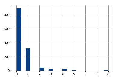
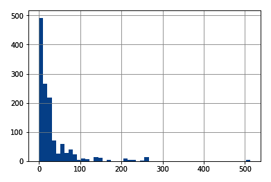
Numerical variables can be discrete or continuous. Discrete variables are those where the pool of possible values is finite and are generally whole numbers, such as 1, 2, and 3. Examples of discrete variables include the number of children, number of pets, or the number of bank accounts. Continuous variables are those whose values may take any number within a range. Examples of continuous variables include the price of a product, income, house price, or interest rate. Categorical variables are values that are selected from a group of categories, also called labels. Examples of categorical variables include gender, which takes values of male and female, or country of birth, which takes values of Argentina, Germany, and so on.

In this recipe, we will learn how to identify continuous, discrete, and categorical variables by inspecting their values and the data type that they are stored and loaded with in pandas.

Discrete variables are usually of the int type, continuous variables are usually of the float type, and categorical variables are usually of the object type when they're stored in pandas. However, discrete variables can also be cast as floats, while numerical variables can be cast as objects. Therefore, to correctly identify variable types, we need to look at the data type and inspect their values as well. Make sure you have the correct library versions installed and that you've downloaded a copy of the Titanic dataset, as described in the Technical requirements section.

First, let's import the necessary Python libraries:

1. Load the libraries that are required for this recipe:

import pandas as pd
import matplotlib.pyplot as plt

2. Load the Titanic dataset and inspect the variable types:

data = pd.read_csv('titanic.csv')
data.dtypes

The variable types are as follows:

pclass         int64
survived       int64
name          object
sex           object
age          float64
sibsp          int64
parch          int64
ticket        object
fare         float64
cabin         object
embarked      object
boat          object
body         float64
home.dest     object
dtype: object

3. Inspect the distinct values of the sibsp discrete variable:

data['sibsp'].unique()

The possible values that sibsp can take can be seen in the following code:

array([0, 1, 2, 3, 4, 5, 8], dtype=int64)

data['fare'].unique()[0:20]

array([211.3375, 151.55  ,  26.55  ,  77.9583,   0.    ,  51.4792,
        49.5042, 227.525 ,  69.3   ,  78.85  ,  30.    ,  25.925 ,
       247.5208,  76.2917,  75.2417,  52.5542, 221.7792,  26.    ,
        91.0792, 135.6333])

In this recipe, we identified the variable data types of a publicly available dataset by inspecting the data type in which the variables are cast and the distinct values they take. First, we used pandas read_csv() to load the data from a CSV file into a dataframe. Next, we used pandas dtypes to display the data types in which the variables are cast, which can be float for continuous variables, int for integers, and object for strings. We observed that the continuous variable fare was cast as float, the discrete variable sibsp was cast as int, and the categorical variable embarked was cast as an object. Finally, we identified the distinct values of a variable with the unique() method from pandas. We used unique() together with a range, [0:20], to output the first 20 unique values for fare, since this variable shows a lot of distinct values.

To understand whether a variable is continuous or discrete, we can also make a histogram:

1. Let's make a histogram for the sibsp variable by dividing the variable value range into 20 intervals:

data['sibsp'].hist(bins=20)

The output of the preceding code is as follows:

Note how the histogram of a discrete variable has a broken, discrete shape.

2. Now, let's make a histogram of the fare variable by sorting the values into 50 contiguous intervals:

data['fare'].hist(bins=50)

The output of the preceding code is as follows:

The histogram of continuous variables shows values throughout the variable value range.

For more details on pandas and variable types, check out https://pandas.pydata.org/pandas-docs/stable/getting_started/basics.html#basics-dtypes.

For details on other variables in the Titanic dataset, check the accompanying Jupyter Notebook in this book's GitHub repository (https://github.com/PacktPublishing/Python-Feature-Engineering-Cookbook).