Regularization

When a model is ill-conditioned or prone to overfitting, regularization offers some valid tools to mitigate the problems. From a mathematical viewpoint, a regularizer is a penalty added to the cost function, to impose an extra condition on the evolution of the parameters:

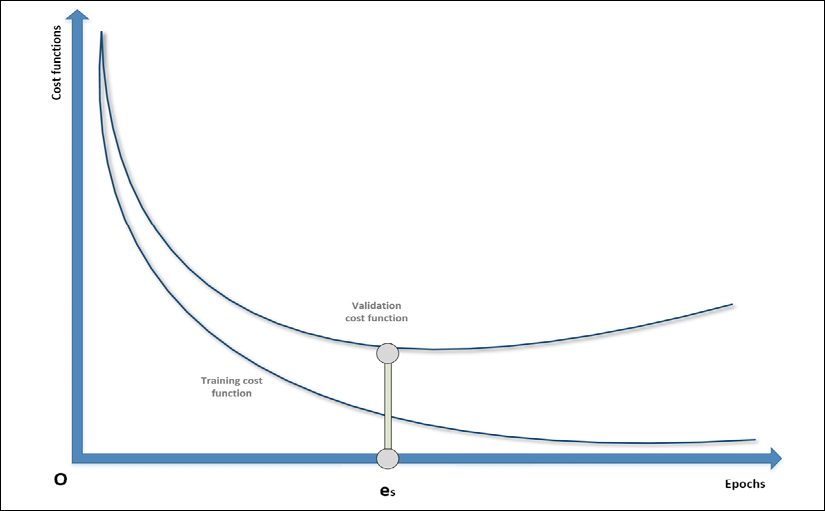
The parameter controls the strength of the regularization, which is expressed through the function . A fundamental condition on is that it must be differentiable so that the new composite cost function can still be optimized using SGD algorithms. In general, any regular function can be employed; however, we normally need a function that can contrast the indefinite growth of the parameters.

To understand the principle, let's consider the following diagram:

Interpolation with a linear curve (left) and a parabolic one (right)

In the first diagram, the model is linear and has two parameters, while in the second one, it is quadratic and has three parameters. We already know that the second option is more prone to overfitting, but if we apply a regularization term, it's possible to avoid the growth of the first quadratic parameter and transform the model into a linearized version.

Of course, there's a difference between choosing a lower-capacity model and applying a regularization constraint. In the first case, we are renouncing the possibility offered by the extra capacity with a consequent risk of large bias, while with regularization we keep the same model but optimize it to reduce the variance and only slightly increase the bias. I hope it's clear that regularization always leads to a suboptimal model M' and, in particular, if the original M is unbiased, M' will be biased proportionally to and to the kind of regularization used.

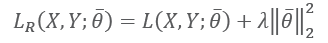
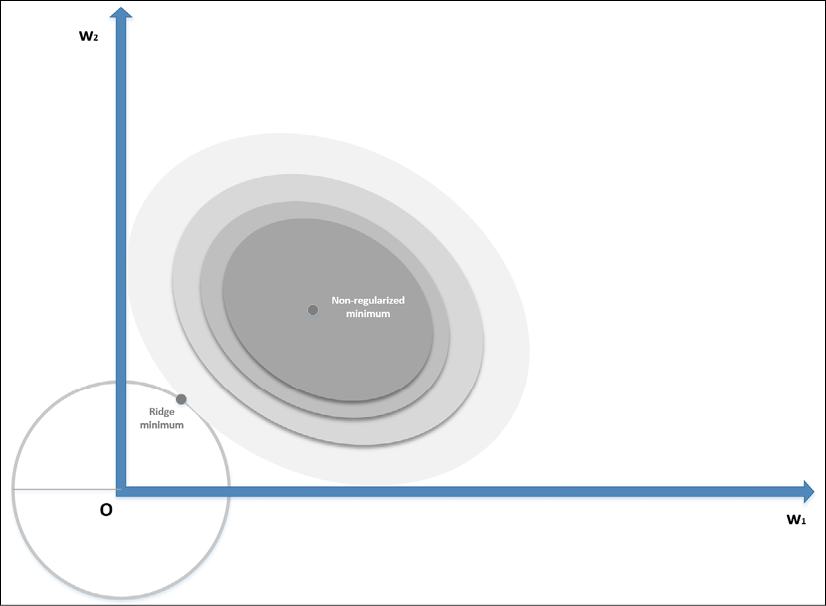
Generally speaking, if the absolute minimum of a cost function with respect to a training set is c_opt, any model with c > c_opt is suboptimal. This means that the training error is larger, but the generalization error might be better controlled.

In fact, a perfectly trained model could have learned the structure of the training set and reached a minimum loss, but, when a new sample is checked, the performance is much worse.

Even if it's not very mathematically rigorous, we can say that regularization often acts as a brake that avoids perfect convergence. By doing this, it keeps the model in a region where the generalization error is lower, which is, generally, the main objective of machine learning. Hence, this extra penalty can be accepted in the context of the bias-variance trade-off.

A small bias can be acceptable when it's the consequence of a drastic variance reduction (that is, a smaller generalization error); however, I strongly suggest that you don't employ regularization as a black-box technique, but instead to check (for example, using cross-validation) which value yields the optimal result, intended as a trade-off.

Examples of Regularization Techniques

At this point, we can explore the most common regularization techniques and discuss their properties.

L₂ or Ridge regularization

L₂ or Ridge regularization, also known as Tikhonov regularization, is based on the squared L₂-norm of the parameter vector:

This penalty avoids infinite growth of the parameters—for this reason, it's also known as weight shrinkage—and it's particularly useful when the model is ill-conditioned, or there is multicollinearity due to the fact that the samples are not completely independent, which is a relatively common condition.

In the following diagram, we see a schematic representation of the Ridge regularization in a bidimensional scenario:

 

Ridge (L₂) regularization

The zero-centered circle represents the Ridge boundary, while the shaded surface is the original cost function. Without regularization, the minimum (w₁, w₂) has a magnitude (for example, the distance from the origin) which is about double the one obtained by applying a Ridge constraint, confirming the expected shrinkage.

When applied to regressions solved with the Ordinary Least Squares (OLS) algorithm, it's possible to prove that there always exists a Ridge coefficient, so that the weights are shrunk with respect to the OLS ones. The same result, with some restrictions, can be extended to other cost functions.

Moreover, Andrew Ng (in Ng A. Y., Feature selection, L1 vs. L2 regularization, and rotational invariance, ICML, 2004) proved that L₂ regularization, applied to the majority of classification algorithms, allows us to obtain rotational invariance. In other words, if the training set is rotated, a regularized model will yield the same prediction distribution as the original one. Another fundamental aspect to remember is that L₂-regularization shrinks the weights independent of the scale of the data. Therefore, if the features have different scales, the result may be worse than expected.

It's easy to understand this concept by considering a simple linear model with two variables, y = ax₁ + bx₁ + c. As the L₂ has a single control coefficient, the effect will be the same on both a and b (excluding the intercept c). If and , the shrinkage will affect x₁ much more than x₂.

For this reason, we recommend scaling the dataset before applying the regularization. Other important properties of this method will be discussed throughout the book, when specific algorithms are introduced.

L₁ or Lasso regularization

L₁ or Lasso regularization is based on the L₁-norm of the parameter vector:

While Ridge shrinks all the weights inversely proportionally to their importance, Lasso can shift the smallest weight to zero, creating a sparse parameter vector.

The mathematical proof is beyond the scope of this book; however, it's possible to understand it intuitively by considering the following bidimensional diagram:

Lasso (L₁) regularization

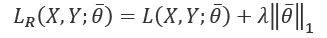
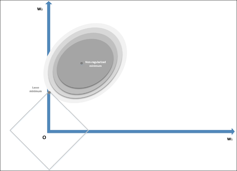
The zero-centered square represents the Lasso boundaries in a bidimensional scenario (it will be a hyperdiamond in ). If we consider a generic line, the probability of that line being tangential to the square is higher at the corners, where at least one parameter is null—exactly one parameter in a bidimensional scenario. In general, if we have a vectorial convex function f(x) (we provide a definition of convexity in Chapter 7, Advanced Clustering and Unsupervised Models), we can define:

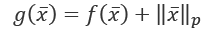
As any L_p-norm is convex, as well as the sum of convex functions, is also convex. The regularization term is always non-negative, and therefore the minimum corresponds to the norm of the null vector.

When minimizing , we also need to consider the contribution of the gradient of the norm in the ball centered in the origin, where the partial derivatives don't exist. Increasing the value of p, the norm becomes smoothed around the origin, and the partial derivatives approach zero for .

On the other hand, excluding the L₀-norm and all the norms with allows an even stronger sparsity, but is non-convex (even if L₀ is currently employed in the quantum algorithm QBoost). With p = 1 the partial derivatives are always +1 or -1, according to the sign of . Therefore, it's easier for the L₁-norm to push the smallest components to zero, because the contribution to the minimization (for example, with gradient descent) is independent of x_i, while an L₂-norm decreases its speed when approaching the origin.

This is a non-rigorous explanation of the sparsity achieved using the L₁-norm. In practice, we also need to consider the term , which bounds the value of the global minimum; however, it may help the reader to develop an intuitive understanding of the concept. It's possible to find further, more mathematically rigorous details in Sra S., Nowozin S., Wright S. J. (edited by), Optimization for Machine Learning, The MIT Press, 2011.

Lasso regularization is particularly useful when a sparse representation of a dataset is needed. For example, we could be interested in finding the feature vectors corresponding to a group of images. As we expect to have many features, but only a subset of those features present in each image, applying the Lasso regularization allows us to force all the smallest coefficients to become null, which helps us by suppressing the presence of the secondary features.

Another potential application is latent semantic analysis, where our goal is to describe the documents belonging to a corpus in terms of a limited number of topics. All these methods can be summarized in a technique called sparse coding, where the objective is to reduce the dimensionality of a dataset by extracting the most representative atoms, using different approaches to achieve sparsity.

Another important property of L₁ regularization concerns its ability to perform an implicit feature selection, induced by the sparsity. In a generic scenario, a dataset can also include irrelevant features that don't contribute to increasing the accuracy of the classification. This can happen because real-world datasets are often redundant, and the data collectors are more interested in their readability than in their usage for analytical purposes. There are many techniques (some of them are described in Bonaccorso G., Machine Learning Algorithms, Second Edition, Packt, 2018) that can be employed to select only those features that really transport unique pieces of information and discard the remaining ones; however, L₁ is particularly helpful.

First of all, it's automatic and no preprocessing steps are required. This is extremely useful in deep learning. Moreover, as Ng pointed out in the aforementioned paper, if a dataset contains n features, the minimum number of samples required to increase the accuracy over a predefined threshold is affected by the logarithm of the number of redundant or irrelevant features.

This means, for example, that if dataset X contains 1000 points and the optimal accuracy is achieved with this sample size when all the features are informative when k < p features are irrelevant, we need approximately 1000 + O(log k) samples. This is a simplification of the original result; for example, if p = 5000 and 500 features are irrelevant, assuming the simplest case, we need about data points.

Such a result is very important because it's often difficult and expensive to obtain a large number of new samples, in particular when they are obtained in experimental contexts (for example, social sciences, pharmacological research, and so on). Before moving on, let's consider a synthetic dataset containing 500 points with only five informative features:

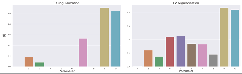
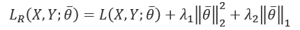
from sklearn.datasets import make_classification
from sklearn.preprocessing import StandardScaler
X, Y = make_classification(n_samples=500, n_classes=2, n_features=10, n_informative=5, 
                           n_redundant=3, n_clusters_per_class=2, random_state=1000)
ss = StandardScaler()
X_s = ss.fit_transform(X)

We can now fit two logistic regression instances with the whole dataset: the first one using the L₂ regularization and the second one using L₁. In both cases, the strength is kept fixed:

from sklearn.linear_model import LogisticRegression
lr_l2 = LogisticRegression(solver='saga', penalty='l2', C=0.25, random_state=1000)
lr_l1 = LogisticRegression(solver='saga', penalty='l1', C=0.25, random_state=1000)
lr_l2.fit(X_s, Y)
lr_l1.fit(X_s, Y)

It's possible to see that, in both cases, the 10-fold cross-validation yields approximately the same average accuracy. However, in this case, we are more interested in checking the feature selection properties of L₁; therefore we are going to compare the 10 coefficients of the two models, available as an instance variable coef_. The results are shown in the following figure:

Logistic regression coefficients with L1 (left) and L2 (right) regularizations

As you can see, L₂ regularization tends to shrink all coefficients almost uniformly, excluding the dominance of 9 and 10, while L₁ performs a feature selection, by keeping only 5 non-null coefficients. This result is coherent with the structure of the dataset, in that it contains only 5 informative features and, therefore, a good classification algorithm can get rid of the remaining ones.

It's helpful to remember that we often need to create explainable models. That is to say, we often need to create models whose output can be immediately traced back to its causes. When there are many parameters, this task becomes more difficult. The usage of Lasso allows us to exclude all those features whose importance is secondary with respect to a primary group. In this way, the resulting model is smaller, and definitely more explainable.

As a general suggestion, in particular when working with linear models, I invite the reader to perform a feature selection to remove all non-determinant factors; and L₁ regularization is an excellent choice that avoids an additional preprocessing step.

Having discussed the main properties of both L₁ and L₂ regularizations, we can now explain how to combine them in order to exploit the respective benefits.

ElasticNet

In many real cases, it's useful to apply both Ridge and Lasso regularization in order to force weight shrinkage and a global sparsity. It is possible by employing the ElasticNet regularization, defined as:

The strength of each regularization is controlled by the parameters and . ElasticNet can yield excellent results whenever it's necessary to mitigate overfitting effects, while encouraging sparsity. We're going to apply all these regularization techniques when we discuss deep learning architectures.

Early stopping

Even though it's a pure regularization technique, early stopping is often considered a last resort when all other approaches to prevent overfitting, and maximize validation accuracy, fail. In many cases, above all in deep learning scenarios even though it can also happen with SVMs and other simpler classifiers, it's possible to observe a typical behavior of the training process, considering both training and the validation cost functions:

Example of early stopping before the beginning of the ascending phase of a U-curve

During the first epochs, both costs decrease, but it can happen that after a threshold epoch e_s, the validation cost starts increasing. If we continue with the training process, this results in overfitting the training set and increasing the variance.

For this reason, when there are no other options, it's possible to prematurely stop the training process. In order to do so, it's necessary to store the last parameter vector before the beginning of a new iteration and, in the case of no improvements or the accuracy worsening, to stop the process and recover the last set of parameters.

As explained, this procedure must never be considered as the best choice, because a better model or an improved dataset could yield higher performances. With early stopping, there's no way to verify alternatives, therefore it must be adopted only at the last stage of the process and never at the beginning.

Many deep learning frameworks such as Keras include helpers to implement early stopping callbacks. However, it's important to check whether the last parameter vector is the one stored before the last epoch or the one corresponding to e_s. In this case, it could be helpful to repeat the training process, stopping it at the epoch previous to e_s, where the minimum validation cost has been achieved.