Understanding the impact of the learning rate

In order to understand how learning rate impacts the training of a model, let's consider a very simple case, where we try to fit the following equation (note that the following equation is different from the toy dataset that we have been working on so far):

Note that y is the output and x is the input. With a set of input and expected output values, we will try and fit the equation with varying learning rates to understand the impact of the learning rate.

1. We specify the input and output dataset as follows:

x = [[1],[2],[3],[4]]
y = [[3],[6],[9],[12]]

2. Define the feed_forward function. Further, in this instance, we will modify the network in such a way that we do not have a hidden layer and the architecture is as follows:

Note that, in the preceding function, we are estimating the parameters w and b:

from copy import deepcopy
import numpy as np
def feed_forward(inputs, outputs, weights):
    pred_out = np.dot(inputs,weights[0])+ weights[1]
    mean_squared_error = np.mean(np.square(pred_out \
                                           - outputs))
    return mean_squared_error

3. Define the update_weights function just like we defined it in the Gradient descent in code section:

def update_weights(inputs, outputs, weights, lr):
    original_weights = deepcopy(weights)
    org_loss = feed_forward(inputs, outputs,original_weights)
    updated_weights = deepcopy(weights)
    for i, layer in enumerate(original_weights):
        for index, weight in np.ndenumerate(layer):
            temp_weights = deepcopy(weights)
            temp_weights[i][index] += 0.0001
            _loss_plus = feed_forward(inputs, outputs, \
                                      temp_weights)
            grad = (_loss_plus - org_loss)/(0.0001)
            updated_weights[i][index] -= grad*lr
    return updated_weights

4. Initialize weight and bias values to a random value:

W = [np.array([[0]], dtype=np.float32), 
     np.array([[0]], dtype=np.float32)]

Note that the weight and bias values are randomly initialized to values of 0. Further, the shape of the input weight value is 1 x 1, as the shape of each data point in the input is 1 x 1 and the shape of the bias value is 1 x 1 (as there is only one node in the output and each output has one value).

5. Let's leverage the update_weights function with a learning rate of 0.01, loop through 1,000 iterations, and check how the weight value (W) varies over increasing epochs:

weight_value = []
for epx in range(1000):
    W = update_weights(x,y,W,0.01)
    weight_value.append(W[0][0][0])

Note that, in the preceding code, we are using a learning rate of 0.01 and repeating the update_weights function to fetch the modified weight at the end of each epoch. Further, in each epoch, we gave the most recent updated weight as an input to fetch the updated weight in the next epoch.

6. Plot the value of the weight parameter at the end of each epoch:

import matplotlib.pyplot as plt
%matplotlib inline
epochs = range(1, 1001)
plt.plot(epochs,weight_value)
plt.title('Weight value over increasing \
epochs when learning rate is 0.01')
plt.xlabel('Epochs')
plt.ylabel('Weight value')

The preceding code results in a variation in the weight value over increasing epochs as follows:

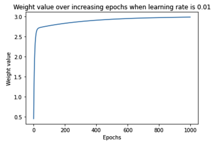
Note that, in the preceding output, the weight value gradually increased in the right direction and then saturated at the optimal value of ~3.

In order to understand the impact of the value of the learning rate on arriving at the optimal weight values, let's understand how weight value varies over increasing epochs when the learning rate is 0.1 and when the learning rate is 1.

The following charts are obtained when we modify the corresponding learning rate value in step 5 and execute step 6 (the code to generate the following charts is the same as the code we learned earlier, with a change in the learning rate value, and is available in the associated notebook in GitHub):

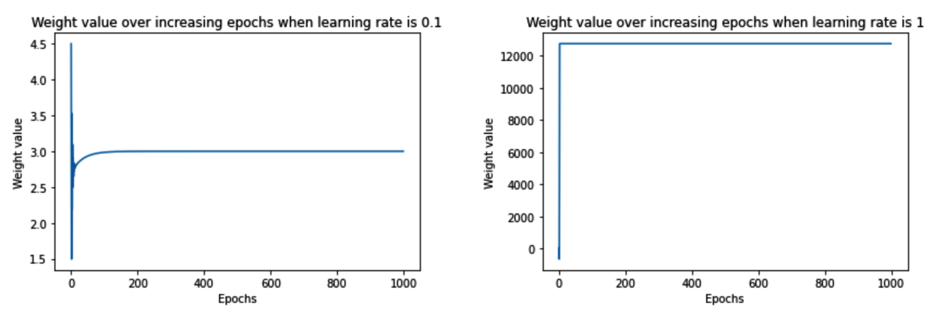
Note that when the learning rate was very small (0.01), the weight value moved slowly (over a higher number of epochs) towards the optimal value. However, with a slightly higher learning rate (0.1), the weight value oscillated initially and then quickly saturated (in fewer epochs) to the optimal value. Finally, when the learning rate was high (1), the weight value spiked to a very high value and was not able to reach the optimal value.

The reason the weight value did not spike by a large amount when the learning rate was low is that we restricted the weight update by an amount that was equal to the gradient * learning rate, essentially resulting in a small amount of weight update when the learning rate was small. However, when the learning rate was high, weight update was high, after which the change in loss (when the weight was updated by a small value) was so small that the weight could not achieve the optimal value.

In order to have a deeper understanding of the interplay between the gradient value, learning rate, and weight value, let's run the update_weights function only for 10 epochs. Further, we will print the following values to understand how they vary over increasing epochs:

• Weight value at the start of each epoch
• Loss prior to weight update
• Loss when the weight is updated by a small amount
• Gradient value

We modify the update_weights function to print the preceding values as follows:

def update_weights(inputs, outputs, weights, lr):
    original_weights = deepcopy(weights)
    org_loss = feed_forward(inputs, outputs, original_weights)
    updated_weights = deepcopy(weights)
    for i, layer in enumerate(original_weights):
        for index, weight in np.ndenumerate(layer):
            temp_weights = deepcopy(weights)
            temp_weights[i][index] += 0.0001
            _loss_plus = feed_forward(inputs, outputs, \
                                      temp_weights)
            grad = (_loss_plus - org_loss)/(0.0001)
            updated_weights[i][index] -= grad*lr
            if(i % 2 == 0):
                print('weight value:', \
                      np.round(original_weights[i][index],2), \
                      'original loss:', np.round(org_loss,2), \
                      'loss_plus:', np.round(_loss_plus,2), \
                      'gradient:', np.round(grad,2), \
                      'updated_weights:', \
                      np.round(updated_weights[i][index],2))
    return updated_weights

The lines highlighted in bold font in the preceding code are where we modified the update_weights function from the previous section, where, first, we are checking whether we are currently working on the weight parameter by checking if (i % 2 == 0) as the other parameter corresponds to the bias value, and then we are printing the original weight value (original_weights[i][index]), loss (org_loss), updated loss value (_loss_plus), gradient (grad), and the resulting updated weight value (updated_weights).

Let's now understand how the preceding values vary over increasing epochs across the three different learning rates that we are considering:

• Learning rate of 0.01: We will check the values using the following code:

W = [np.array([[0]], dtype=np.float32), 
     np.array([[0]], dtype=np.float32)]
weight_value = []
for epx in range(10):
    W = update_weights(x,y,W,0.01)
    weight_value.append(W[0][0][0])
print(W)
import matplotlib.pyplot as plt
%matplotlib inline
epochs = range(1, 11)
plt.plot(epochs,weight_value)
plt.title('Weight value over increasing \
epochs when learning rate is 0.01')
plt.xlabel('Epochs')
plt.ylabel('Weight value')

The preceding code results in the following output:

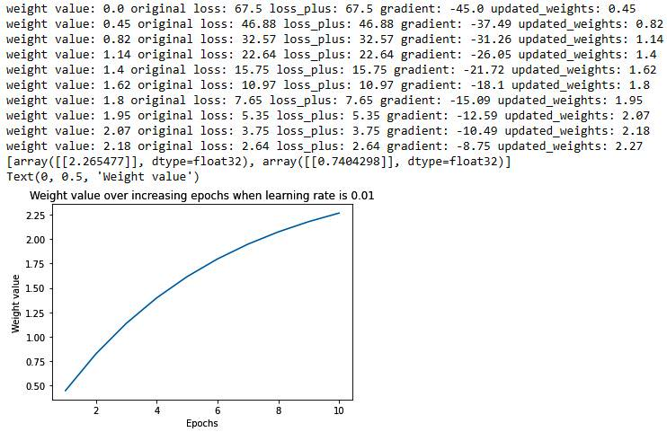
Note that, when the learning rate was 0.01, the loss value decreased slowly, and also the weight value updated slowly towards the optimal value. Let's now understand how the preceding varies when the learning rate is 0.1.

• Learning rate of 0.1: The code remains the same as in the learning rate of 0.01 scenario, however, the learning rate parameter would be 0.1 in this scenario. The output of running the same code with the changed learning rate parameter value is as follows:

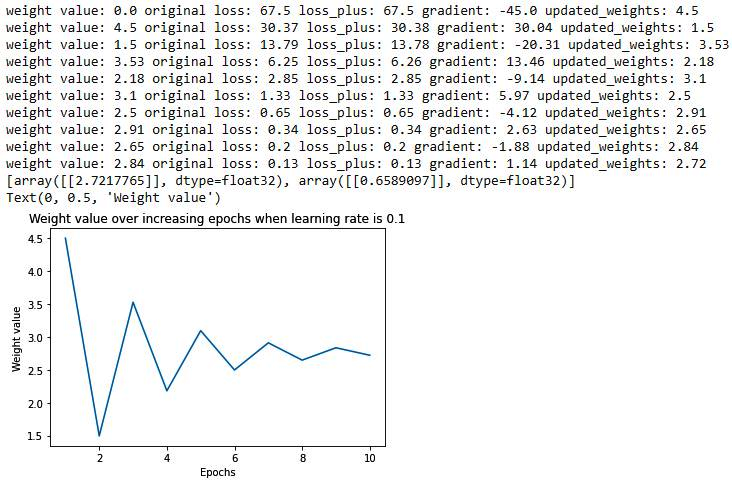
Let's contrast the learning rate scenarios of 0.01 and 0.1 – the major difference between the two is as follows:

When the learning rate was 0.01, the weight updated much slower when compared to a learning rate of 0.1 (from 0 to 0.45 in the first epoch when the learning rate is 0.01, to 4.5 when the learning rate is 0.1). The reason for the slower update is the lower learning rate as the weight is updated by the gradient times the learning rate.

In addition to the weight update magnitude, we should note the direction of the weight update:

The gradient is negative when the weight value is smaller than the optimal value while it is positive when the weight value is larger than the optimal value. This phenomenon helps in updating weight values in the right direction.

Finally, we will contrast the preceding with a learning rate of 1:

• Learning rate of 1: The code remains the same as in the learning rate of 0.01 scenario, however, the learning rate parameter would be 1 in this scenario. The output of running the same code with the changed learning rate parameter is as follows:

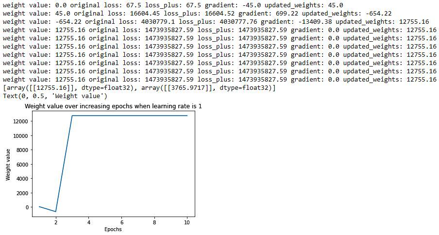
From the preceding diagram, we can see that the weight has deviated to a very high value (as at the end of the first epoch, the weight value is 45, which further deviated to a very large value in later epochs). In addition to that, the weight value moved to a very large amount, so that a small change in the weight value hardly results in a change in the gradient, and hence the weight got stuck at that high value.

Now that we have learned about the building blocks of a neural network – feedforward propagation, backpropagation, and learning rate, in the next section, we will summarize a high-level overview of how these three are put together to train a neural network.