

When working with large amounts of data, it can become difficult to locate blank spaces within the spreadsheet. Blank spaces can cause numerous issues including errors and breaks in formatting.
In this recipe, you will learn to locate and highlight all blanks within your data.
Smaller spreadsheets may allow you to quickly locate missed or blank information; however, Excel provides an automated method for performing this task that becomes increasingly more helpful with larger data-sets.
1. Under the Home tab click on the option Find & Select, and then choose Go To Special.

2. In the Go To Special... dialog box that opens, select the option for blank and click on OK.

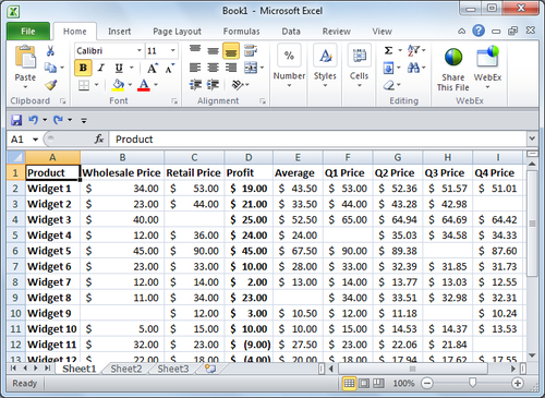
3. All of the blanks within the data have now been highlighted.

4. Select a format for the blank cells, such as filling them with a color such as yellow. This now provides a contrasting visual indicator to locate blanks on the screen or when printed.

The Go To Special... option under Excel's built-in find feature provides several criteria that you can select to find data within your spreadsheet. By selecting blanks, Excel quickly parsed through the data and located and selected all the cells that contained no data. With all of the blank cells selected, you can easily apply a visual indicator.
While this recipe added a yellow fill to indicate blank cells, you can easily add other indicators such as lines, characters, and so on, which may provide for easier printing.
For further control of the formatting options used within this recipe, conditional formatting may provide a more automated, albeit, more involved method of locating and identifying blanks or other data. For more information on the use of conditional formatting, see the recipe Making printing easier to read.