

Extracting word representations
What does a word mean to a computer? What about an image or an audio file? To put it simply, nothing. A computer circuit can only process signals that contain two voltage levels or states, similar to an on-off switch. This representation is the well-known binary system where every quantity is expressed as a sequence of 1s (high voltage) and 0s (low voltage). For example, the number 1001 in binary is 9 in decimal (the numerical system humans employ). Computers utilize this representation to encode the pixels of an image, the samples of an audio file, a word, and much more, as illustrated in Figure 2.3:
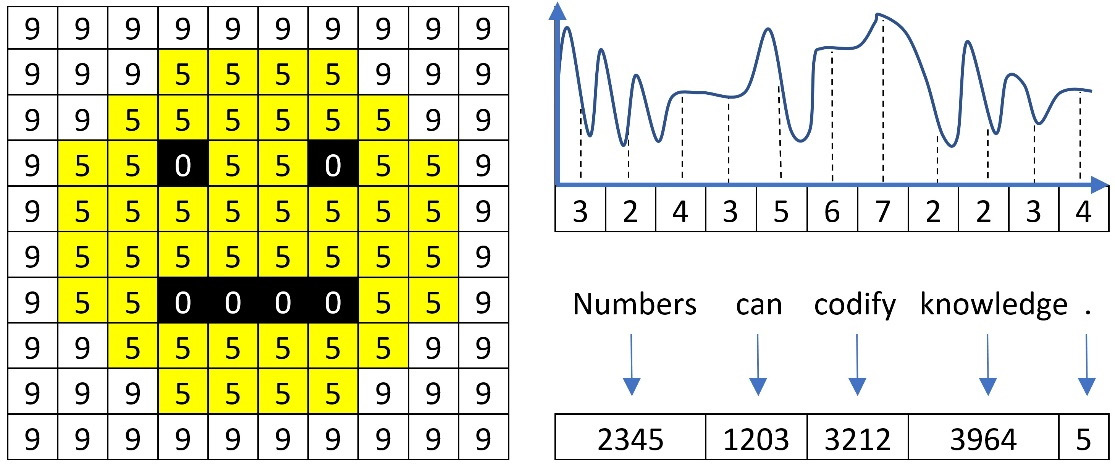
Figure 2.3 – Image pixels, audio samples, and words represented with numbers
Based on this representation, our computers can make sense of the data and process it the way we wish, such as by rendering an image on the screen, playing an audio track, or translating an input sentence into another language. As the book focuses on text, we will learn about the standard approaches for representing words in a piece of text data. More advanced techniques are a subject in the subsequent chapters.
Using label encoding
In ML problems, there are various ways to represent words; label encoding is the simplest form. For example, consider this quote from Aristotle: a friend to all is a friend to none. Using the label-encoding scheme and a dictionary with words to indices (a:0, all:1, friend:2, is:3, none:4, to:5), we can produce the mapping shown in Table 2.2:
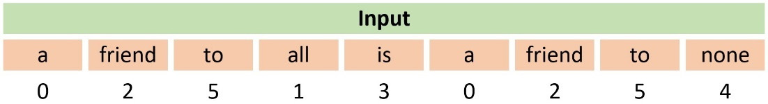
Table 2.2 – An example of using label encoding
We observe that a numerical sequence replaces the words in the sentence. For example, the word friend maps to the number 2. In Python, we can use the LabelEncoder class from the sklearn module and feed it with the quote from Aristotle:
from sklearn.preprocessing import LabelEncoder
# Create the label encoder and fit it with data.
labelencoder = LabelEncoder()
labelencoder.fit(["a", "all", "friend", "is", "none", "to"])
# Transform an input sentence.
x = labelencoder.transform(["a", "friend", "to", "all", "is", "a", "friend", "to", "none"])
print(x)
>> [0 2 5 1 3 0 2 5 4]
The output is the same array as the one in Table 2.2. There is a caveat, however. When an ML algorithm uses this representation, it implicitly considers and tries to exploit some kind of order among the words, for example, a<friend<to (because 0 < 2 < 5). This order does not exist in reality. On the other hand, label encoding is appropriate if there is an ordinal association between the words. For example, the good, better, and best triplet can be encoded as 1, 2, and 3, respectively. Another example is online surveys, where we frequently use categorical variables with predefined values for each question, such as disagree=-1, neutral=0, and agree=+1. In these cases, label encoding can be more appropriate, as the associations good<better<best and disagree<neutral<agree make sense.
Using one-hot encoding
Another well-known word representation technique is one-hot encoding, which codifies every word as a vector with zeros and a single one. Notice that the position of the one uniquely identifies a specific word; consequently, no two words exist with the same one-hot vector. Table 2.3 shows an example of this representation using the previous input sentence from Aristotle:
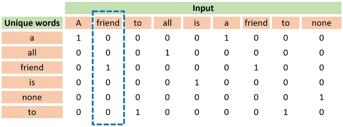
Table 2.3 – An example of using one-hot encoding
Observe that the first column in the table includes all unique words. The word friend appears at position 3, so its one-hot vector is [0, 0, 1, 0, 0, 0]. The more unique words in a dataset, the longer the vectors are because they depend on the vocabulary size.
In the code that follows, we use the OneHotEncoder class from the sklearn module:
from sklearn.preprocessing import OneHotEncoder
# The input.
X = [['a'], ['friend'], ['to'], ['all'], ['is'], ['a'], ['friend'], ['to'], ['none']]
# Create the one-hot encoder.
onehotencoder = OneHotEncoder()
# Fit and transform.
enc = onehotencoder.fit_transform(X).toarray()
print(enc.T)
>> [[1. 0. 0. 0. 0. 1. 0. 0. 0.]
 [0. 0. 0. 1. 0. 0. 0. 0. 0.]
 [0. 1. 0. 0. 0. 0. 1. 0. 0.]
 [0. 0. 0. 0. 1. 0. 0. 0. 0.]
 [0. 0. 0. 0. 0. 0. 0. 0. 1.]
 [0. 0. 1. 0. 0. 0. 0. 1. 0.]]
Looking at the code output, can you identify a drawback to this approach? The majority of the elements in the array are zeros. As the corpus size increases, so does the vocabulary size of the unique words. Consequently, we need bigger one-hot vectors where all other elements are zero except for one. Matrixes of this kind are called sparse and can pose challenges due to the memory required to store them.
Next, we examine another approach that addresses both ordinal association and sparsity issues.
Using token count encoding
Token count encoding, also known as the Bag-of-Words (BoW) representation, counts the absolute frequency of each word within a sentence or a document. The input is represented as a bag of words without taking into account grammar or word order. This method uses a Term Document Matrix (TDM) matrix that describes the frequency of each term in the text. For example, in Table 2.4, we calculate the number of times a word from a minimal vocabulary of seven words appears in Aristotle’s quote:
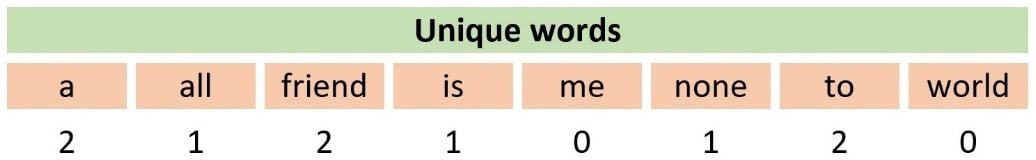
Table 2.4 – An example of using token count encoding
Notice that the corresponding cell in the table contains the value 0 when no such word is present in the quote. In Python, we can convert a collection of text documents to a matrix of token counts using the CountVectorizer class from the sklearn module, as shown in the following code:
from sklearn.feature_extraction.text import CountVectorizer
# The input.
X = ["a friend to all is a friend to none"]
# Create the count vectorizer.
vectorizer = CountVectorizer(token_pattern='[a-zA-Z]+')
# Fit and transform.
x = vectorizer.fit_transform(X)
print(vectorizer.vocabulary_)
>> {'a': 0, 'friend': 2, 'to': 5, 'all': 1, 'is': 3, 'none': 4}
Next, we print the token counts for the quote:
print(x.toarray()[0])
>> [2 1 2 1 1 2]
The CountVectorizer class takes the token pattern argument as the input [a-zA-Z]+, which identifies words with lowercase or uppercase letters. Don’t worry if the syntax of this pattern is not yet clear. We are going to demystify it later in the chapter. In this case, the code informs us that the word a (with id 0) appears twice, and therefore the first element in the output array [2, 1, 2, 1, 1, 2] is 2. Similarly, the word none, the fifth element of the array, appears once.
We can continue by extending the vectorizer using a property of human languages: the fact that certain word combinations are more frequent than others. We can verify this characteristic by performing Google searches of various word combinations inside double quotation marks. Each one yields a different number of search results, an indirect measure of their frequency in language.
When reading a spam email, we don’t usually focus on isolated words and instead identify patterns in word sequences that trigger an alert in our brain. How can we leverage this fact in our spam detection problem? One possible answer is to use n-grams as tokens for CountVectorizer. In simple terms, n-grams illustrate word sequences, and due to their simplicity and power, they have been extensively used in Natural Language Processing (NLP) applications. There are different variants of n-grams depending on the number of words that we group; for a single word, they are called unigrams; for two words, bigrams, and three words trigrams. Figure 2.4 presents the first three order n-grams for Aristotle’s quote:
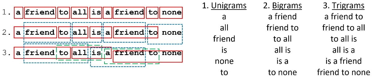
Figure 2.4 – Unigrams, bigrams, and trigrams for Aristotle’s quote
We used unigrams in the previous Python code, but we can now add the ngram_range argument during the vectorizer construction and use bigrams instead:
from sklearn.feature_extraction.text import CountVectorizer
# The input.
X = ["a friend to all is a friend to none"]
# Create the count vectorizer using bi-grams.
vectorizer = CountVectorizer(ngram_range=(2,2), token_pattern='[a-zA-Z]+')
# Fit and transform.
x = vectorizer.fit_transform(X)
print(vectorizer.vocabulary_)
>> {'a friend': 0, 'friend to': 2, 'to all': 4, 'all is': 1, 'is a': 3, 'to none': 5}
Next, we print the token counts for the quote:
print(x.toarray()[0])
>> [2 1 2 1 1 1]
In this case, the friend to bigram with an ID of 2 appears twice, so the third element in the output array is 2. For the same reason, the to none bigram (the last element) appears only once.
In this section, we discussed how to utilize word frequencies to encode a piece of text. Next, we will present a more sophisticated approach that uses word frequencies differently. Let’s see how.
Using tf-idf encoding
One limitation of BoW representations is that they do not consider the value of words inside the corpus. For example, if solely frequency were of prime importance, articles such as a or the would provide the most information for a document. Therefore, we need a representation that penalizes these frequent words. The remedy is the term frequency-inverse document frequency (tf-idf) encoding scheme that allows us to weigh each word in the text. You can consider tf-idf as a heuristic where more common words tend to be less relevant for most semantic classification tasks, and the weighting reflects this approach.
From a virtual dataset with 10 million emails, we randomly pick one containing 100 words. Suppose that the word virus appears three times in this email, so its term frequency (tf) is  . Moreover, the same word appears in 1,000 emails in the corpus, so the inverse document frequency (idf) is equal to
  . The tf-idf weight is simply the product of these two statistics:
  . We reach a high tf-idf weight when we have a high frequency of the term in the random email and a low document frequency of the same term in the whole dataset. Generally, we calculate tf-idf weights with the following formula:
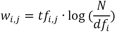
Where:
 Weight of word i in document j
 Frequency of word i in document j
 Total number of documents
 Number of documents containing word i
Performing the same calculations in Python is straightforward. In the following code, we use TfidfVectorizer from the sklearn module and a dummy corpus with four short sentences:
from sklearn.feature_extraction.text import TfidfVectorizer
# Create a dummy corpus.
corpus = [
        'We need to meet tomorrow at the cafeteria.',
        'Meet me tomorrow at the cafeteria.',
        'You have inherited millions of dollars.',
        'Millions of dollars just for you.']
# Create the tf-idf vectorizer.
vectorizer = TfidfVectorizer()
# Generate the tf-idf matrix.
tfidf = vectorizer.fit_transform(corpus)
Next, we print the result as an array:
print(tfidf.toarray())
>> [[0.319  0.319    0.       0.      0.       0.
  0.        0.       0.319    0.      0.404    0.
  0.319     0.404    0.319    0.404   0.]
 [0.388     0.388    0.       0.      0.       0.
  0.        0.493    0.388    0.      0.       0.
  0.388     0.       0.388    0.      0.]
 [0.        0.       0.372    0.      0.472    0.472
  0.        0.       0.       0.372   0.       0.372
  0.        0.       0.       0.      0.372]
 [0.        0.       0.372    0.472   0.       0.
  0.472     0.       0.       0.372   0.    0.372
  0.        0.       0.       0.      0.372]]
What does this output tell us? Each of the four sentences is encoded with one tf-idf vector of 17 elements (this is the number of unique words in the corpus). Non-zero values show the tf-idf weight for a word in the sentence, whereas a value equal to zero signifies the absence of the specific word. If we could somehow compare the tf-idf vectors of the examples, we can tell which pair resembles more. Undoubtedly, 'You have inherited millions of dollars.' is closer to 'Millions of dollars just for you.' than the other two sentences. Can you perhaps guess where this discussion is heading? By calculating an array of weights for all the words in an email, we can compare it with the reference arrays of spam or non-spam and classify it accordingly. The following section will tell us how.
Calculating vector similarity
Mathematically, there are different ways to calculate vector resemblances, such as cosine similarity (cs) or Euclidean distance. Specifically, cs is the degree to which two vectors point in the same direction, targeting orientation rather than magnitude (see Figure 2.5).
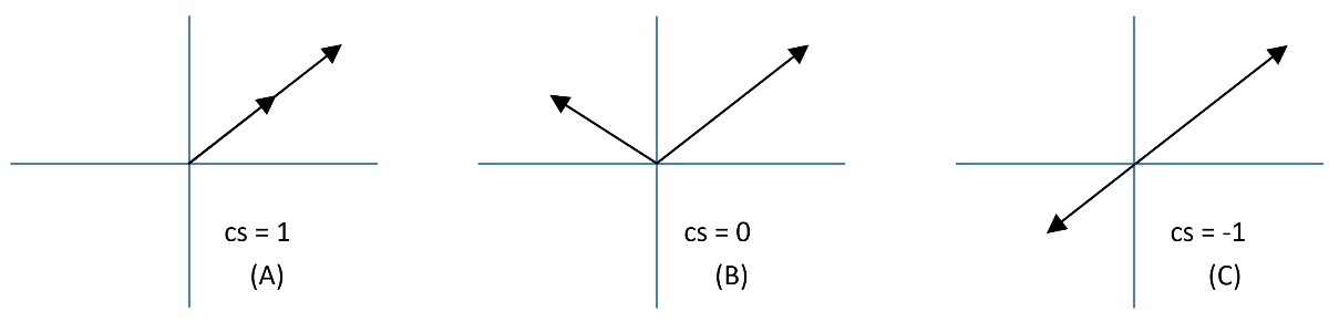
Figure 2.5 – Three cases of cosine similarity
When the two vectors point in the same direction, the cs equals 1 (in A in Figure 2.5); when they are perpendicular, it is 0 (in B in Figure 2.5), and when they point in opposite directions, it is -1 (in C in Figure 2.5). Notice that only values between 0 to 1 are valid in NLP applications since the term frequencies cannot be negative.
Consider now an example where A, B, and C are vectors with three elements each, so that A = (4, 4, 4), B = (1, 7, 5), and C = (-5, 5, 1). You can think of each number in the vector as a coordinate in an xyz-space. Looking at Figure 2.6, A and B seem more similar than C. Do you agree?
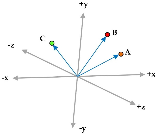
Figure 2.6 – Three vectors A, B, and C in a three-dimensional space
We calculate the dot product (signified with the symbol •) between two vectors of the same size by multiplying their elements in the same position.  and
and  are two vectors, so their dot product is
  . In our example,
 and
and  . Additionally, the magnitude of the vector
  is defined as
 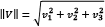 and in our case,
 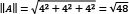 ,
,  , and
, and  .
.
Therefore, we obtain the following:
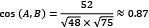 ,
, 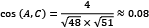 , and
, and 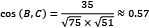 .
.
The results confirm our first hypothesis that A and B are more similar than C.
In the following code, we calculate the cs of the tf-idf vectors between the corpus’s first and second examples:
from sklearn.metrics.pairwise import cosine_similarity
# Convert the matrix to an array.
tfidf_array = tfidf.toarray()
# Calculate the cosine similarity between the first amd second example.
print(cosine_similarity([tfidf_array[0]], [tfidf_array[1]]))
>> [[0.62046087]]
We also repeat the same calculation between all tf-idf vectors:
# Calculate the cosine similarity among all examples.
print(cosine_similarity(tfidf_array))
>> [[1.         0.62046     0.        0.        ]
 [0.62046       1.          0.        0.        ]
 [0.            0.          1.        0.5542    ]
 [0.            0.          0.5542    1.        ]]
As expected, the value between the first and second examples is high and equal to 0.62. Between the first and the third example, it is 0, 0.55 between the third and the fourth, and so on.
Exploring tf-idf has concluded our discussion on the standard approaches for representing text data. The importance of this step should be evident, as it relates to the machine’s ability to create models that better understand textual input. Failing to get good representations of the underlying data typically leads to suboptimal results in the later phases of analysis. We will also encounter a powerful representation technique for text data in Chapter 3, Classifying Topics of Newsgroup Posts.
In the next section, we will go a step further and discuss different techniques of preprocessing data that can boost the performance of ML algorithms.