With significant enhancements in the quality and quantity of algorithms in recent years, this second edition of Hands-On Reinforcement Learning with Python has been revamped into an example-rich guide to learning state-of-the-art reinforcement learning (RL) and deep RL algorithms with TensorFlow 2 and the OpenAI Gym toolkit.
In addition to exploring RL basics and foundational concepts such as Bellman equation, Markov decision processes, and dynamic programming algorithms, this second edition dives deep into the full spectrum of value-based, policy-based, and actor-critic RL methods. It explores state-of-the-art algorithms such as DQN, TRPO, PPO and ACKTR, DDPG, TD3, and SAC in depth, demystifying the underlying math and demonstrating implementations through simple code examples.
The book has several new chapters dedicated to new RL techniques, including distributional RL, imitation learning, inverse RL, and meta RL. You will learn to leverage stable baselines, an improvement of OpenAI’s baseline library, to effortlessly implement popular RL algorithms. The book concludes with an overview of promising approaches such as meta-learning and imagination augmented agents in research.
By the end, you will become skilled in effectively employing RL and deep RL in your real-world projects.
We have learned that Gym provides a variety of environments for training a reinforcement learning agent. To clearly understand how the Gym environment is designed, we will start with the basic Gym environment. After that, we will understand other complex Gym environments.
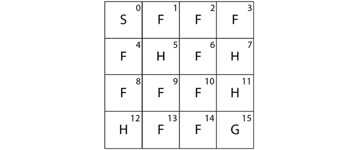
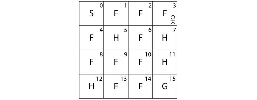
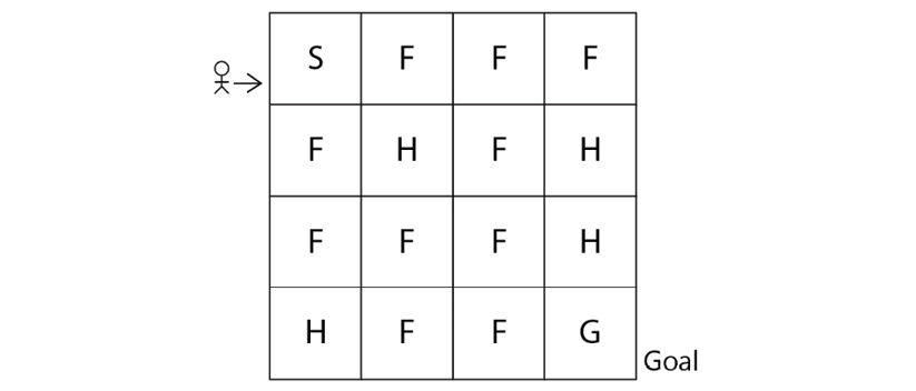
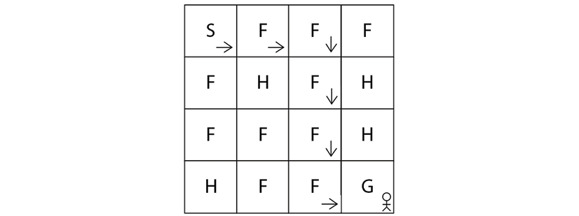
Let's introduce one of the simplest environments called the Frozen Lake environment. Figure 2.1 shows the Frozen Lake environment. As we can observe, in the Frozen Lake environment, the goal of the agent is to start from the initial state S and reach the goal state G:
Figure 2.1: The Frozen Lake environment
In the preceding environment, the following apply:
S denotes the starting state
F denotes the frozen state
H denotes the hole state
G denotes the goal state
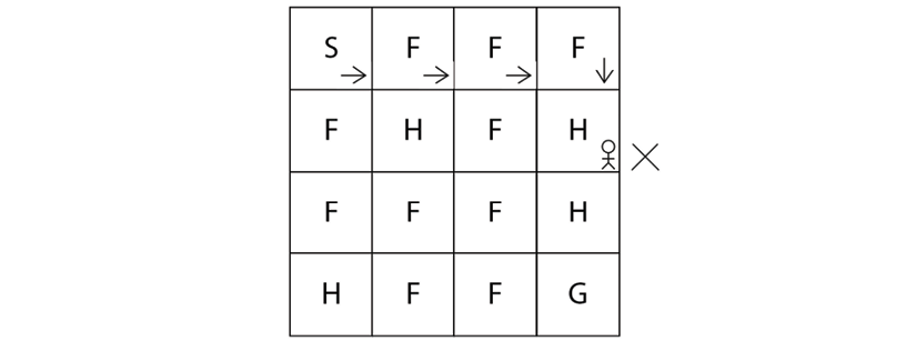
So, the agent has to start from state S and reach the goal state G. But one issue is that if the agent visits state H, which is the hole state, then the agent will fall into the hole and die as shown in Figure 2.2:
Figure 2.2: The agent falls down a hole
So, we need to make sure that the agent starts from S and reaches G without falling into the hole state H as shown in Figure 2.3:
Figure 2.3: The agent reaches the goal state
Each grid box in the preceding environment is called a state, thus we have 16 states (S to G) and we have 4 possible actions, which are up, down, left, and right. We learned that our goal is to reach the state G from S without visiting H. So, we assign +1 reward for the goal state G and 0 for all other states.
Thus, we have learned how the Frozen Lake environment works. Now, to train our agent in the Frozen Lake environment, first, we need to create the environment by coding it from scratch in Python. But luckily we don't have to do that! Since Gym provides various environments, we can directly import the Gym toolkit and create a Frozen Lake environment.
Now, we will learn how to create our Frozen Lake environment using Gym. Before running any code, make sure that you have activated our virtual environment universe. First, let's import the Gym library:
import gym
Next, we can create a Gym environment using the make function. The make function requires the environment id as a parameter. In Gym, the id of the Frozen Lake environment is FrozenLake-v0. So, we can create our Frozen Lake environment as follows:
env = gym.make("FrozenLake-v0")
After creating the environment, we can see how our environment looks like using the render function:
env.render()
The preceding code renders the following environment:
Figure 2.4: Gym's Frozen Lake environment
As we can observe, the Frozen Lake environment consists of 16 states (S to G) as we learned. The state S is highlighted indicating that it is our current state, that is, the agent is in the state S. So whenever we create an environment, an agent will always begin from the initial state, which in our case is state S.
That's it! Creating the environment using Gym is that simple. In the next section, we will understand more about the Gym environment by relating all the concepts we have learned in the previous chapter.
Exploring the environment
In the previous chapter, we learned that the reinforcement learning environment can be modeled as a Markov decision process (MDP) and an MDP consists of the following:
States: A set of states present in the environment.
Actions: A set of actions that the agent can perform in each state.
Transition probability: The transition probability is denoted by . It implies the probability of moving from a state s to the state while performing an action a.
Reward function: The reward function is denoted by . It implies the reward the agent obtains moving from a state s to the state while performing an action a.
Let's now understand how to obtain all the above information from the Frozen Lake environment we just created using Gym.
States
A state space consists of all of our states. We can obtain the number of states in our environment by just typing env.observation_space as follows:
print(env.observation_space)
The preceding code will print:
Discrete(16)
It implies that we have 16 discrete states in our state space starting from state S to G. Note that, in Gym, the states will be encoded as a number, so the state S will be encoded as 0, state F will be encoded as 1, and so on as Figure 2.5 shows:
Figure 2.5: Sixteen discrete states
Actions
We learned that the action space consists of all the possible actions in the environment. We can obtain the action space by using env.action_space:
print(env.action_space)
The preceding code will print:
Discrete(4)
It shows that we have 4 discrete actions in our action space, which are left, down, right, and up. Note that, similar to states, actions also will be encoded into numbers as shown in Table 2.1:
Table 2.1: Four discrete actions
Transition probability and reward function
Now, let's look at how to obtain the transition probability and the reward function. We learned that in the stochastic environment, we cannot say that by performing some action a, the agent will always reach the next state exactly because there will be some randomness associated with the stochastic environment, and by performing an action a in the state s, the agent reaches the next state with some probability.
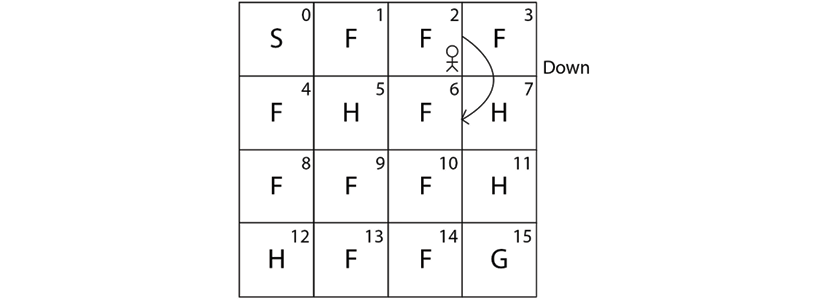
Let's suppose we are in state 2 (F). Now, if we perform action 1 (down) in state 2, we can reach state 6 as shown in Figure 2.6:
Figure 2.6: The agent performing a down action from state 2
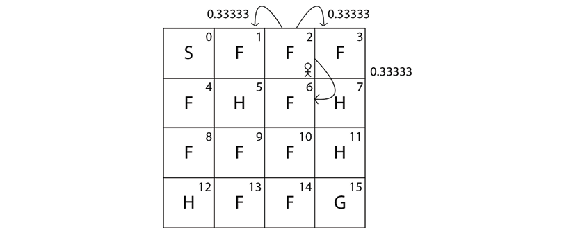
Our Frozen Lake environment is a stochastic environment. When our environment is stochastic, we won't always reach state 6 by performing action 1 (down) in state 2; we also reach other states with some probability. So when we perform an action 1 (down) in state 2, we reach state 1 with probability 0.33333, we reach state 6 with probability 0.33333, and we reach state 3 with probability 0.33333 as shown in Figure 2.7:
Figure 2.7: Transition probability of the agent in state 2
As we can see, in a stochastic environment we reach the next states with some probability. Now, let's learn how to obtain this transition probability using the Gym environment.
We can obtain the transition probability and the reward function by just typing env.P[state][action]. So, to obtain the transition probability of moving from state S to the other states by performing the action right, we can type env.P[S][right]. But we cannot just type state S and action right directly since they are encoded as numbers. We learned that state S is encoded as 0 and the action right is encoded as 2, so, to obtain the transition probability of state S by performing the action right, we type env.P[0][2] as the following shows:
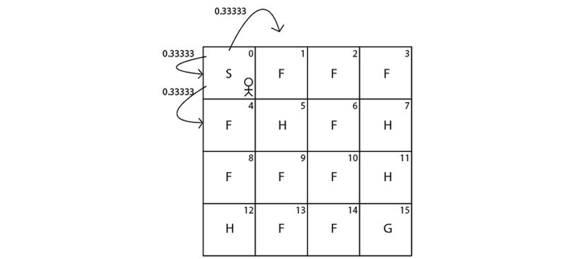
What does this imply? Our output is in the form of [(transition probability, next state, reward, Is terminal state?)]. It implies that if we perform an action 2 (right) in state 0 (S) then:
We reach state 4 (F) with probability 0.33333 and receive 0 reward.
We reach state 1 (F) with probability 0.33333 and receive 0 reward.
We reach the same state 0 (S) with probability 0.33333 and receive 0 reward.
Figure 2.8 shows the transition probability:
Figure 2.8: Transition probability of the agent in state 0
Thus, when we type env.P[state][action], we get the result in the form of [(transition probability, next state, reward, Is terminal state?)]. The last value is Boolean and tells us whether the next state is a terminal state. Since 4, 1, and 0 are not terminal states, it is given as false.
The output of env.P[0][2] is shown in Table 2.2 for more clarity:
Table 2.2: Output of env.P[0][2]
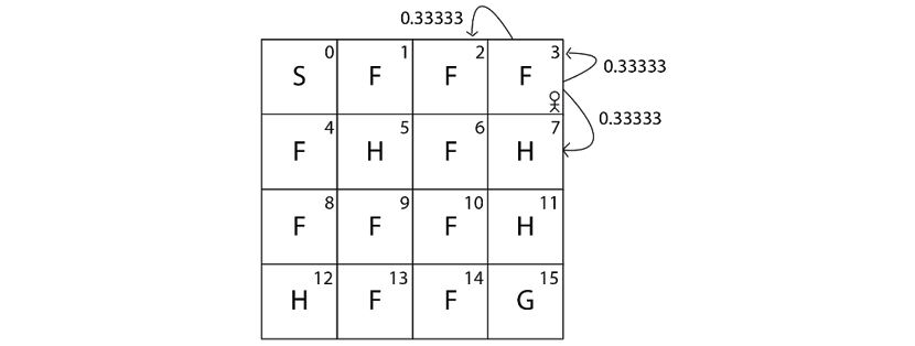
Let's understand this with one more example. Let's suppose we are in state 3 (F) as Figure 2.9 shows:
Figure 2.9: The agent in state 3
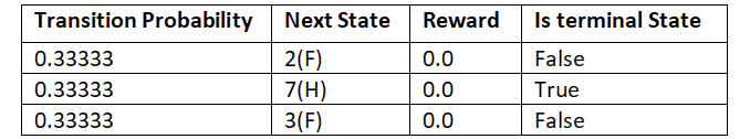
Say we perform action 1 (down) in state 3 (F). Then the transition probability of state 3 (F) by performing action 1 (down) can be obtained as the following shows:
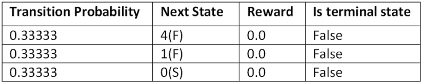
As we learned, our output is in the form of [(transition probability, next state, reward, Is terminal state?)]. It implies that if we perform action 1 (down) in state 3 (F) then:
We reach state 2 (F) with probability 0.33333 and receive 0 reward.
We reach state 7 (H) with probability 0.33333 and receive 0 reward.
We reach the same state 3 (F) with probability 0.33333 and receive 0 reward.
Figure 2.10 shows the transition probability:
Figure 2.10: Transition probabilities of the agent in state 3
The output of env.P[3][1] is shown in Table 2.3 for more clarity:
Table 2.3: Output of env.P[3][1]
As we can observe, in the second row of our output, we have (0.33333, 7, 0.0, True), and the last value here is marked as True. It implies that state 7 is a terminal state. That is, if we perform action 1 (down) in state 3 (F) then we reach state 7 (H) with 0.33333 probability, and since 7 (H) is a hole, the agent dies if it reaches state 7 (H). Thus 7(H) is a terminal state and so it is marked as True.
Thus, we have learned how to obtain the state space, action space, transition probability, and the reward function using the Gym environment. In the next section, we will learn how to generate an episode.
Generating an episode in the Gym environment
We learned that the agent-environment interaction starting from an initial state until the terminal state is called an episode. In this section, we will learn how to generate an episode in the Gym environment.
Before we begin, we initialize the state by resetting our environment; resetting puts our agent back to the initial state. We can reset our environment using the reset() function as shown as follows:
state = env.reset()
Action selection
In order for the agent to interact with the environment, it has to perform some action in the environment. So, first, let's learn how to perform an action in the Gym environment. Let's suppose we are in state 3 (F) as Figure 2.11 shows:
Figure 2.11: The agent is in state 3 in the Frozen Lake environment
Say we need to perform action 1 (down) and move to the new state 7 (H). How can we do that? We can perform an action using the step function. We just need to input our action as a parameter to the step function. So, we can perform action 1 (down) in state 3 (F) using the step function as follows:
env.step(1)
Now, let's render our environment using the render function:
env.render()
As shown in Figure 2.12, the agent performs action 1 (down) in state 3 (F) and reaches the next state 7 (H):
Figure 2.12: The agent in state 7 in the Frozen Lake environment
Note that whenever we make an action using env.step(), it outputs a tuple containing 4 values. So, when we take action 1 (down) in state 3 (F) using env.step(1), it gives the output as:
(7, 0.0, True, {'prob': 0.33333})
As you might have guessed, it implies that when we perform action 1 (down) in state 3 (F):
We reach the next state 7 (H).
The agent receives the reward 0.0.
Since the next state 7 (H) is a terminal state, it is marked as True.
We reach the next state 7 (H) with a probability of 0.33333.
So, we can just store this information as:
(next_state, reward, done, info) = env.step(1)
Thus:
next_state represents the next state.
reward represents the obtained reward.
done implies whether our episode has ended. That is, if the next state is a terminal state, then our episode will end, so done will be marked as True else it will be marked as False.
info—Apart from the transition probability, in some cases, we also obtain other information saved as info, which is used for debugging purposes.
We can also sample action from our action space and perform a random action to explore our environment. We can sample an action using the sample function:
random_action = env.action_space.sample()
After we have sampled an action from our action space, then we perform our sampled action using our step function:
next_state, reward, done, info = env.step(random_action)
Now that we have learned how to select actions in the environment, let's see how to generate an episode.
Generating an episode
Now let's learn how to generate an episode. The episode is the agent environment interaction starting from the initial state to the terminal state. The agent interacts with the environment by performing some action in each state. An episode ends if the agent reaches the terminal state. So, in the Frozen Lake environment, the episode will end if the agent reaches the terminal state, which is either the hole state (H) or goal state (G).
Let's understand how to generate an episode with the random policy. We learned that the random policy selects a random action in each state. So, we will generate an episode by taking random actions in each state. So for each time step in the episode, we take a random action in each state and our episode will end if the agent reaches the terminal state.
First, let's set the number of time steps:
num_timesteps = 20
For each time step:
for t in range(num_timesteps):
Randomly select an action by sampling from the action space:
random_action = env.action_space.sample()
Perform the selected action:
next_state, reward, done, info = env.step(random_action)
If the next state is the terminal state, then break. This implies that our episode ends:
    if done:
        break
The preceding complete snippet is provided for clarity. The following code denotes that on every time step, we select an action by randomly sampling from the action space, and our episode will end if the agent reaches the terminal state:
import gym
env = gym.make("FrozenLake-v0")
state = env.reset()
print('Time Step 0 :')
env.render()
num_timesteps = 20for t in range(num_timesteps):
random_action = env.action_space.sample()
new_state, reward, done, info = env.step(random_action)
print ('Time Step {} :'.format(t+1))
env.render()
if done:
break
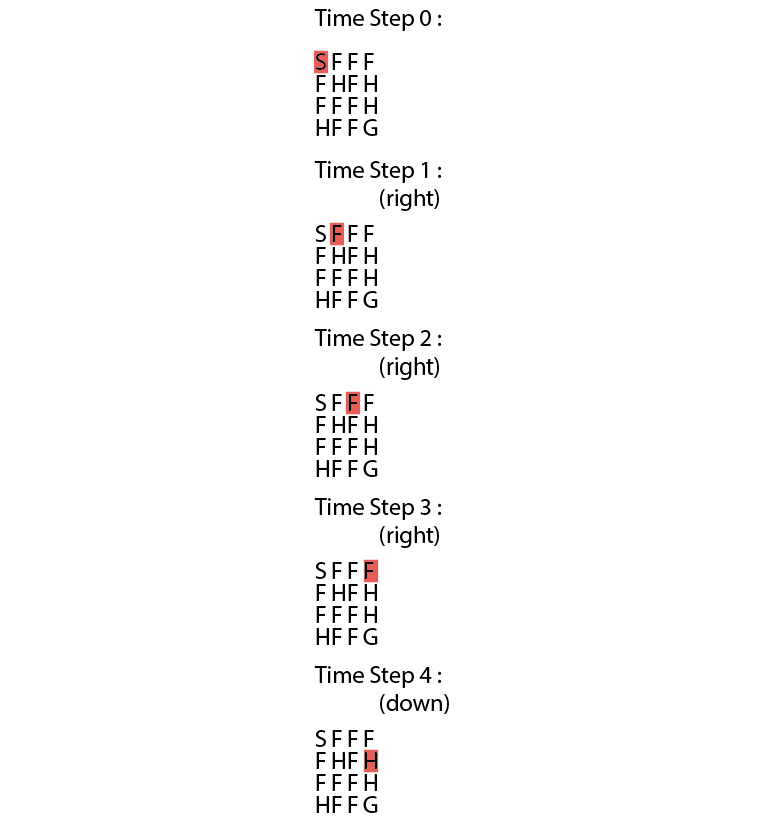
The preceding code will print something similar to Figure 2.13. Note that you might get a different result each time you run the preceding code since the agent is taking a random action in each time step.
As we can observe from the following output, on each time step, the agent takes a random action in each state and our episode ends once the agent reaches the terminal state. As Figure 2.13 shows, in time step 4, the agent reaches the terminal state H, and so the episode ends:
Figure 2.13: Actions taken by the agent in each time step
Instead of generating one episode, we can also generate a series of episodes by taking some random action in each state:
import gym
env = gym.make("FrozenLake-v0")
num_episodes = 10
num_timesteps = 20for i in range(num_episodes):
state = env.reset()
print('Time Step 0 :')
env.render()
for t in range(num_timesteps):
random_action = env.action_space.sample()
new_state, reward, done, info = env.step(random_action)
print ('Time Step {} :'.format(t+1))
env.render()
if done:
break
Thus, we can generate an episode by selecting a random action in each state by sampling from the action space. But wait! What is the use of this? Why do we even need to generate an episode?
In the previous chapter, we learned that an agent can find the optimal policy (that is, the correct action in each state) by generating several episodes. But in the preceding example, we just took random actions in each state over all the episodes. How can the agent find the optimal policy? So, in the case of the Frozen Lake environment, how can the agent find the optimal policy that tells the agent to reach state G from state S without visiting the hole states H?
This is where we need a reinforcement learning algorithm. Reinforcement learning is all about finding the optimal policy, that is, the policy that tells us what action to perform in each state. We will learn how to find the optimal policy by generating a series of episodes using various reinforcement learning algorithms in the upcoming chapters. In this chapter, we will focus on getting acquainted with the Gym environment and various Gym functionalities as we will be using the Gym environment throughout the course of the book.
So far we have understood how the Gym environment works using the basic Frozen Lake environment, but Gym has so many other functionalities and also several interesting environments. In the next section, we will learn about the other Gym environments along with exploring the functionalities of Gym.
Read this chapter and the full book FREE of cost - No Credit card required!
Plus access over 8,000 other expert tech books and videos just by signing up - No commitment!
CONTINUE READING
83
Tech Concepts
36
Programming languages
73
Tech Tools
Unlimited access to the largest independent learning library in tech of over 8,000 expert-authored tech books and videos.
Innovative learning tools, including AI book assistants, code context explainers, and text-to-speech.
50+ new titles added per month and exclusive early access to books as they are being written.


 Free Chapter

 . It implies the probability of moving from a state s to the state
  while performing an action a.
 . It implies the reward the agent obtains moving from a state s to the state
  while performing an action a.