Knowing the basic Julia types for data visualization

This section will explore the Julia syntax, objects, and features that will help us perform data analysis and visualization tasks. Julia and its ecosystem define plenty of object types useful for us when creating visualizations. Because user-defined types are as fast as built-in types in Julia, you are not constrained to using the few structs defined in the language. This section will explore both the built-in and package-defined types that will help us the most throughout this book. But first, let's see how to create and use Julia functions.

Defining and calling functions

A function is an object able to take an input, execute some code on it, and return a value. We have already called functions using the parenthesis syntax – for example, println("Hello World"). We pass the function input values or arguments inside the parentheses that follow the function name.

We can better understand Julia's functions by creating them on our own. Let's make a straightforward function that takes two arguments and returns the sum of them. You can execute the following code in the Julia REPL, inside a new Julia script in VS Code, or into a Jupyter or Pluto cell:

function addition(x, y)

    x + y

end

We can use the function keyword to create a function. We then define its name and declare inside the parentheses the positional and keyword arguments. In this case, we have defined two positional arguments, x, and y. After a new line, we start the function body, which determines the code to be executed by the function. The function body of the previous code contains only one expression – x + y. A Julia function always returns an object, and that object is the value of the last executed expression in the function body. The end keyword indicates the end of the function block.

We can also define the function using the assignation syntax for simple functions such as the previous one, containing only one expression – for example, the following code creates a function that returns the value of subtracting the value of y from x:

subtraction(x, y) = x - y

A Julia function can also have keyword arguments defined by name instead of by position – for example, we used the dir keyword argument when we executed notebook(dir="."). When declaring a function, we should introduce the keyword arguments after a semicolon.

Higher-order functions

Functions are first-class citizens in the Julia language. Therefore, you can write Julia functions that can have other functions as inputs or outputs. Those kinds of functions are called higher-order functions. One example is the sum function, which can take a function as the first argument and apply it to each value before adding them. You can execute the following code to see how Julia takes the absolute value of each number on the vector before adding them:

sum(abs, [-1, 1])

In this example, we used a named function, abs, but usually, the input and output functions are anonymous functions.

Anonymous functions

Anonymous functions are simply functions without a user-defined name. Julia offers two foremost syntaxes to define them, one for single-line functions and the others for multiline functions. The single-line syntax uses the -> operator between the function arguments and its body. The following code will perform sum(abs, [-1, 1]), using this syntax to create an anonymous function as input to sum:

sum(x -> abs(x), [-1, 1])

The other syntax uses the do block to create an anonymous function for a higher-order function, taking a function as the first argument. We can write the previous code in the following way using the do syntax:

sum([-1, 1]) do x

    abs(x)

end

We indicated the anonymous function's arguments after the do keyword and defined the body after a new line. Julia will pass the created anonymous function as the first argument of the higher-order function, which is sum in this case.

Now that we know how to create and call functions, let's explore some types in Julia.

Working with Julia types

You can write Julia types using their literal representations. We have already used some of them throughout the chapter – for example, 2 was an integer literal, and "Hello World" was a string literal. You can see the type of an object using the typeof function – for example, executing typeof("Hello World") will return String, and typeof(2) will return Int64 in a 64-bit operating system or Int32 in a 32-bit one.

In some cases, you will find the dump function helpful, as it shows the type and the structure of an object. We recommend using the Dump function from the PlutoUI package instead, as it works in both Pluto and the Julia REPL – for example, if we execute numbers = 1:5 and then the Dump(numbers) integer literal, we will get the following output in a 64-bit machine:

UnitRange{Int64}

  start: Int64 1

  stop: Int64 5

So, Dump shows that 1:5 creates UnitRange with the start and stop fields, each containing an integer value. You can access those fields using the dot notation – for example, executing numbers.start will return the 1 integer.

Also, note that the type of 1:5 was UnitRange{Int64} in this example. UnitRange is a parametric type, for which Int64 is the value of its type parameter. Julia writes the type parameters between brackets following the type name.

Julia has an advanced type system, and we have learned the basics to explore it. Before learning about some useful Julia types, let's explore one of the reasons for Julia's power – its use of multiple dispatch.

Taking advantage of Julia's multiple dispatch

We have learned how to write functions and to explore the type of objects in Julia. Now, it's time to learn about methods. The functions we have created previously are known as generic functions. As we have not annotated the functions using types, we have also created methods for those generic functions that, in principle, can take objects of any type. You can optionally add type constraints to function arguments. Julia will consider this type annotation when choosing the most specific function method for a given set of parameters. Julia has multiple dispatch, as it uses the type information of all positional arguments to select the method to execute. The power of Julia lies in its multiple dispatch, and plotting packages take advantage of this feature. Let's see what multiple dispatch means by creating a function with two methods, one for strings and the other for integers:

1. Open a Julia REPL and execute the following:

   concatenate(a::String, b::String) = a * b

This code creates a function that concatenates two string objects, a and b. Note that Julia uses the * operator to concatenate strings. We need to use the :: operator to annotate types in Julia. In this case, we are constraining our function to take only objects of the String type.

2. Run concatenate("Hello", "World") to test that our function works as expected; it should return "HelloWorld".
3. Run methods(concatenate) to list the function's methods. You will see that the concatenate function has only one method that takes two objects of the String type – concatenate(a::String, b::String).
4. Execute concatenate(1, 2). You will see that this operation throws an error of the MethodError type. The error tells us that there is no method matching concatenate(::Int64, ::Int64) if we use a 64-bit machine; otherwise, you will see Int32 instead of Int64. The error is thrown because we have defined our concatenate to take only objects of the String type.
5. Execute concatenate(a::Int, b::Int) = parse(Int, string(a) * string(b)) to define a new method for the concatenate function taking two objects of the Int type. The function converts the input integer to strings before concatenation using the string function. Then, it uses parse to get the integer value of the Int type from the concatenated strings.
6. Run methods(concatenate); you will see this time that concatenate has two methods, one for String objects and the other for integers.
7. Run concatenate(1, 2). This time, Julia will find and select the concatenate method taking two integers, returning the integer 12.

Usually, converting types will help you to fix MethodError. When we found the error in step 4 we could have solved it by converting the integers to strings on the call site by running concatenate(string(1), string(2)) to get the "12" string. There are two main ways to convert objects in Julia explicitly – the first is by using the convert function, and the other is by using the type as a function (in other words, calling the type constructor). For example, we can convert 1, an integer, to a floating-point number of 64 bits of the Float64 type using convert(Float64, 1) or Float64(1) – which option is better will depend on the types at hand. For some types, there are special conversion functions; strings are an example of it. We need the string function to convert 1 to "1", as in string(1). Also, converting a string containing a number to that number requires the parse function – for example, to convert "1" to 1, we need to call parse(Int, "1").

At this point, we know the basics for dealing with Julia types. Let's now explore Julia types that will help us create nice visualizations throughout this book.

Representing numerical values

The most classic numbers that you can use are integers and floating-point values. As Julia was designed for scientific computing, it defines number types for different word sizes. The most used ones are Float64, which stores 64-bit floating-point numbers, and Int. This is an alias of Int64 in 64-bit operating systems or Int32 in 32-bit architectures. Both are easy to write in Julia – for example, we have already used Int literals such as -1 and 5. Then, each time you enter a number with a dot, e, or E, it will define Float64 – for example, 1.0, -2e3, and 13.5E10 are numbers of the Float64 type. The dot determines the location of the decimal point and e or E the exponent. Note that .1 is equivalent to 0.1 and 1. is 1.0, as the zero is implicit on those expressions. Float64 has a value to indicate something that is not a number – NaN. When entering numbers in Julia, you can use _ as a digit separator to make the number more legible – for example, 10_000. Sometimes, you need to add units to a number to make it meaningful. In particular, we will use mm, cm, pt, and inch from the Measures package for plotting purposes. After loading that package, write the number followed by the desired unit, for example, 10.5cm. That expression takes advantage of Julia's numeric literal coefficients. Each time you write a numeric literal, such as 10.5, just before a Julia parenthesized expression or variable, such as the cm object, you imply a multiplication. Therefore, writing 10.5cm is equivalent to writing 10.5 * cm; both return the same object.

Representing text

Julia has support for single and multiline string literals. You can write the former using double quotes (") and the latter using triple double quotes ("""). Note that Julia uses single quotes (') to define the literal for single characters of the Char type.

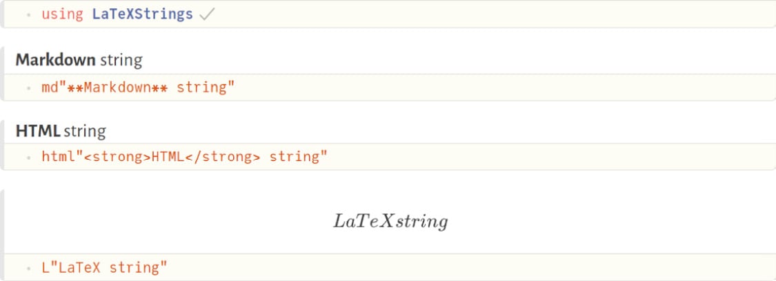
Julia offers other kinds of strings that will be useful for us when creating plots and interactive visualizations – Markdown, HTML, and LaTeX strings. The three of them use Julia's string macros, which you can write by adding a short word before the first quotes – md for Markdown, html for HTML, and L for LaTeX. You will need to load the Markdown standard library to use the md string macro and the LaTeXStrings external package for the L string macro. Note that Pluto automatically loads the Markdown module, so you can use md"..." without loading it. Also, Pluto renders the three of them nicely:

Figure 1.5 – Pluto rendering Markdown, HTML, and LaTeX strings

There is another type associated with text that you will also find in Julia when plotting and analyzing data – symbols. Symbols are interned strings, meaning that Julia stores only one copy of them. You can construct them using a colon followed by a word that should be a valid Julia variable name – for example, :var1. Otherwise, if it is not a valid identifier, you should use String and call the Symbol constructor – for example, Symbol("var1").

Working with Julia collections

We will use two main collection types for data analysis and visualization – tuples and arrays. Julia collections are a broad topic, but we will explore the minimum necessary here. Let's begin with tuples. Tuples are immutable lists of objects of any type that we write between parentheses – for example, ("x", 0) and (1,) are two- and one-element tuples respectively. Note that tuples with one element need the trailing comma.

Arrays can have multiple dimensions; the most common are vectors (one-dimensional arrays) and matrices (two-dimensional arrays). An array is a parametric type that stores the type of elements it contains and the number of dimensions as type parameters. We can construct an array using square brackets – for example, [1] and [1, 2] are vectors with one and two elements respectively. You can also write matrices using square brackets by separating columns with spaces, rather than commas and rows with semicolons or newlines – for example, [1 2; 3 4] is a 2 x 2 matrix.

For arrays, there are also other helpful constructors – zeros, ones, and rand. The three of them take the number of elements to create in each direction – for example, zeros(4, 2) will create a matrix full of zeros with four rows and two columns, while zeros(10) will create a vector of 10 zeros.

Julia offers the colon operator for creating a range of numbers; you can think of them as lazy vectors – for example, we have already seen 1:5 in a previous example. You can collect the elements of a range into a vector using the collect function.

You can index ranges, tuples, and arrays using the squared brackets syntax. Note that Julia has one-based indexing, so the first element of collection will be collection[1].

You can also iterate over ranges, tuples, and arrays. There are two compact ways to iterate through those collections, apply a function, and get a new array. One is using array comprehension – for example, [sqrt(x) for x in 1:5]. Note that comprehension can also have filter expression – for example, if we want the square root only of odd numbers between 1 and 10, we can write [sqrt(x) for x in 1:10 if x % 2 != 0] .

The other compact way to apply a function over each collection element is to use broadcasting. Julia's broadcasting allows applying a function element-wise on arrays of different sizes by expanding singleton dimensions to match their sizes. It also enables operations between scalars and collections. Furthermore, you can use broadcasting to apply a function to a single collection. Note that for each function acting on scalars, Julia doesn't define methods taking collections of them. Therefore, Julia's preferred way to apply such a function to each collection element is to use the dot syntax for broadcasting. You only need to add a dot between the function name and the parentheses on a function call or a dot before an operator – for example, sqrt.(collection) .+ 1. Julia fuses the operations when using this syntax, so the square root and the addition happen in a single iteration.

We have now learned how to work with Julia types, particularly to represent text and numbers and their collections. In the next section, we will use them to create some plots.